The Dutch East India Company and Dutch State Formation in the Seventeenth Century

Introduction

Today firms are part and parcel of the modern capitalist state enterprise. Aside from provisions of the state, firms provide the goods and services people consume, as well as wages (the means of consumption). It is worth asking, then, if early firms had a part in the emergence of the modern state. This paper briefly examines the role of the largest business enterprise of its time, the Dutch East India Company (VOC), in the formation of early-modern Netherlands. It finds that the VOC had an important role in the emergence of an independent Dutch Republic in 1648.

Setting the Stage

The Netherlands, from very early in its history, had a dynamic and varied economy. The Holland region circa 1500 already had the highest urbanization rate in Europe, with 40 percent of labor in early forms of industry, 20 percent in services, 15 percent in fishing and peat digging, supported by a mere 25 percent in agriculture. In addition, it was already dominated by wage labor (at a time when Western Europe on average had only a quarter of its population producing for wages)[1].

Politically the Dutch Republic was unique. From its outset in the tenth century free peasants inhabited the region with property rights over their land, relatively lax feudal structures were in place, and nobility were weak.[2]

During the latter stages of the Middle Ages the merchant class began to secure control of the town and municipal councils in the provinces of Holland and Zeeland. This process was exacerbated during the opening years of the Eighty Years’ War when Sea-Beggars retook coastal towns from Spain and placed themselves at the head of the councils. There was considerable variation in political control, however. Regions like Guelderland and Friesland, for example, remained in the hands of the nobility and landowning farmers.

In 1568 war broke out with Spain. By 1579 the Seventeen Provinces of the Netherlands, first brought together under Charles V in 1543, were split. The southern provinces, having been substantially decimated by battles with Spain, had already pledged allegiance to the Habsburg Spanish King Phillip II. The northern states, meanwhile, united around William of Orange and banded together as the Republic of Seven United Provinces under the Union of Utrecht in 1579, were intent on fighting the Spanish.

There are, then, many occasions across history one could point to as the founding of the Dutch State. For the purposes of this paper we will take this founding event to be the Treaty of Münster in 1648. This is not at all unreasonable. Prior to this period, though seven states had come together to form the Dutch Republic, the future of the Republic was very much in doubt. The war with Spain consumed considerable resources and it was not at all clear the Dutch union would emerge independent of Spain as it did at the end of the Eighty Years’ War. Indeed, 1648 seems to be the consensus of scholars as to when the Dutch State first arose. This choice also facilitates an examination of how the Dutch East India Company, what would become the world’s largest business enterprise, aided in the Dutch Republic’s founding.

Emergence of the VOC

Seaborne exploration in the Netherlands has a long and rich history dating back to the High Middle Ages when fishing arose as a significant part of the early Dutch economy. By 1565 the Baltic trading fleet already numbered 700 ships and by the last decade of the sixteenth century approximately 12 ships per year sailed as far afield as Italy. Even West Africa saw 20 Dutch ships per year by 1600. But as trade pushed toward southern Africa, and further still toward Asia, additional costs–such as increased provisions and heavy artillery to fight privateers–quickly made funding by standard methods prohibitive. [3]

Traditionally, each voyage of a particular ship constituted its own “firm” (or rederij), with several partners coming together with equity shares sometimes down to the 1/128^th ownership fraction. Ships traveling further east, however, were four times as expensive and took at least twice as long to return, increasing risk for investors. Sub-shares began being sold to friends and family, but an even more permanent enterprise was required for true success. In 1602 the States-General persuaded several existing partnerships to come together and form the The Dutch East India Company—or Vereenigde Oost-Indische Compagnie in Dutch (hereafter referred to simply as “VOC” ). By 1607, after four rounds of equity financing, investment in the VOC stood at 9 million guilders.[4]

By the seventeenth century town and municipal councils had come to be largely controlled by the merchant class. This in turn meant that the States-General, the national governing body, was also largely influenced by merchants. The VOC, then, was an institution created by merchants for merchants. It was a State before the Dutch Republic itself had acquired full statehood. The VOC could enter into treaties, enlist soldiers and wage war, and build fortresses and outposts abroad. This gave it unrivalled economic freedom as well as the substantial political power that came with the profits.

There were three economic contributions the VOC made toward the formation of the Dutch State: increased liquidity in capital markets, the emergence of Amsterdam as the central European hub for information exchange, and general economic stimulus through employment and colonization efforts. All three led toward state formation through roughly the same means: helping to fund the Eighty Years’ War against Spain.

Increased Liquidity

Firms in early seventeenth century Netherlands had two primary forms of raising funds. The first type was the dividing of equity shares. These were split between two or three, but up to 15, partners. The second form of fundraising was IOU issuance (essentially an early form of corporate bond). By 1600 these debt issuances varied in amount from 600 to 3,000 guilders and ranged from three to 12 months.[5]

The problem was that neither method was particularly liquid. Information asymmetries made the price of finding the probable success of a particular shipping venture costly. Since early operations were small, there was a perceived risk about whether the returning vessel would be loaded with enough tradable goods to recoup the initial costs and have enough leftover for interest payments. This hindered the development of a market for buyers of both the equity and debt financing.

This changed with the formation of the VOC. Share-ownership was split substantially more than previously, with about 1,100 initial subscribers in Amsterdam (which had a population of only 50,000)[6]. Perhaps more importantly, the VOC established a set of procedures to transfer ownership between parties. Shares were easily tradable by means of double-entry registration in the company’s ledger. What resulted was the Bourse, the world’s first stock exchange. The exchange led to the use of shares as collateral for loans on the money market, reducing transaction costs over other forms of collateral such as commodities. Indeed, from 1602 to 1620 interest rates on short-term debt dropped from nearly eight percent to 5.5 percent.[7] The primary cause of this drop was two-fold. The first reason was the increased liquidity of financing instruments described above. The second was an increase in capital availability as merchants immigrated to Amsterdam; this phenomenon was itself likely caused, in some part, by the rise of the VOC.

With time the Bourse grew and, along with the Dutch Central Bank founded in 1609, played an important part in maintaining Dutch credit. The availability of Dutch debt financing persisted even as Dutch borrowing continued and war expenditures crested at 13 million florins (90 percent of total outlays).[8]

Amsterdam as an Information Exchange

The VOC also improved the information gathering and dissemination of sixteenth century Amsterdam, helping it to become the key information hub of Europe. This is no small economic contribution. As W. Fritschy noted in his book on the early Dutch economy, “Economic historians have long stressed that assembly and exchange of business information are important parts of the operation of a commercial center.”[9]

The VOC made three important contributions in the area of information networking. First, the VOC, in an attempt to streamline its operations in marketing, ordering, and price setting, began compiling information from its vast overseas network of colonial outposts. Later, it hired correspondents specifically to fill the role of information reporter.[10] Second, the VOC aided in the distribution of information. The directors of the VOC, the so-called “Heeren XVII”, and other high-level company officers, were often members of the political merchant oligarchy. As members of this commercial group, they would share information coming in from abroad with other elites who would in turn share it with their friends and family, and so on. Information would then spread down through the commercial classes until it became common knowledge. Third, in an attempt to forecast commodity prices, seasonal and yearly variations in importation of goods, and supply and demand across Europe at large, the VOC instituted a process of archival record keeping. As with other types of information, the forecasts that were rendered from studying these archives became public knowledge. Even today there are about 4,000 meters of shelved VOC archival documents worldwide.[11]

General Economic Stimulus

The VOC was a massive organization, especially for its day, and as such was large enough to have a substantial effect on the larger Dutch economy. Between 1602 and 1796, 1,772 ships made 4,785 passages to outposts in the “East Indies.” Over these two hundred years nearly one million Europeans rode aboard its fleet for short- or long-term visits to southern Africa and Asia. At its height 3,000 VOC employees worked in the Dutch Republic at offices, warehouses, and shipyards while 12,000 seamen manned its fleet.[12] In total, more than 2.5 million tons of goods from Asia were brought back for trade. (Compare this to the VOC’s nearest competitor, The British East India Company, which carried only one-fifth the total tonnage on traffic of 2,690 ships)[13]. In addition, the substantial number of colonial outposts established by the VOC no doubt acted to project Dutch power abroad, transforming it into a world power.

The VOC was truly the behemoth of the world’s commercial trading system during these two centuries. Profits came with its success. From 1630 to 1730 the average annual profit was 2 million guilders, of which fifty to seventy-five percent were distributed as dividends with the remainder being reinvested.[14]

Although it is not possible to know the exact magnitude of the VOC’s effects on the Dutch economy on the whole, it no doubt had a substantial impact. The rise of the VOC paralleled a gradual rise in living standards for the average worker. Yearly income of urban day-laborers rose from 195 florins in 1600 to 292 by 1650, and from 270 to 384 for the middle class worker.[15] This in turn paralleled a steadily increasing reliance on tax revenue that, along with government debt, helped to fund the war with Spain.

VOC Political Control

It is clear that the VOC had a powerful positive impact on the Dutch economy and as a result helped it to rise ever further above the Malthusian trap, a process Francis Fukuyama identified as a prerequisite for state development. Additionally, it aided directly in the surge in the Dutch economy that kept credit flowing and incomes, and therefore tax revenue, rising. All of this is simply to say that, despite being part of a broader and richer network of economic and trading activity, the VOC in particular seems to have played an important role in funding the war against Spain and thus ensuring the establishment of a Dutch State.

The VOC’s influence, however, did not end with the economy. The Heeren XVII and other VOC shareholders were extraordinarily prominent in Dutch politics. In fact, the VOC felt so empowered that in 1644 the company told the States-General that:

“The places and strongholds which they had captured in the East Indies should not be regarded as national conquests but as the property of private merchants, who were entitled to sell those places to whomsoever they wished, even if it was to the King of Spain, or to some other enemy of the United Provinces.”[16]

The VOC, with this quite remarkable declaration, demonstrated it felt supremely confident with its preeminence within the wider Dutch system. This is likely because the States-General themselves had chartered the company years earlier and bestowed it with such broad latitude. This political influence was magnified by the rather prominent position of Holland, and in particular Amsterdam (home of the main VOC office), in broader Dutch political decision-making.

In theory, the Seven Provinces of the Dutch Republic were each autonomous and sovereign with the House of Orange acting as stadtholder responsible mostly for military affairs. The Dutch Republic has often been thought of as an exception to the standard pattern of divine right monarchical or absolutist centralization as a prerequisite for state formation. And it was certainly an exception to the model of prolonged war leading to strong centralized government as it did in Western Europe. In fact, the States-General had essential no national political authority to do things like impose a national tax—this was done at the provincial level. In practice, however, Holland came to fill the role of the central authority.

This stemmed simply from its substantial economic contribution to the Republic. Nominally, Holland carried a “mere” 58 percent of the Dutch Republic’s financial burden, but in practice its sway equated to far more.[17] This gave the region increased negotiating power—if a particular policy was to be implemented, Holland must first be convinced. For alas, if Holland happened to disagree, the autonomous nature of the confederation allowed for the province to simply boycott implementation. But this in turn would almost certainly prohibit funding for the policy since invariably Holland would end up footing the bill for any legislation that passed.

Within these various levels of municipal, provincial, and national government sat the VOC’s directors, officers, and shareholders. These groups were so influential in Dutch politics (indeed often they were the very same people) that it caused an anonymous pamphleteer to famously protest:

“For, they say, if we complain to the regents of the VOC and the magistrates of the towns, there sit the directors [the Heeren XVII], […] if to the admiralties, there are the directors again. If to the Estates General, we find that they and the directors are sitting there together at the same time.”[18]

The famous Johan de Witt, for example, known as “the first Dutch Statesman” for his leadership leading up to and during the Anglo-Dutch wars, was the largest shareholder in the Zeeland chamber of the VOC.[19]

The VOC was economically and politically the single most important Dutch enterprise and conducted the bulk of its business in Holland, which itself supplied the majority of wealth and tax revenue to the Dutch Republic and had the political sway to prove it. It stands to reason, therefore, that aside from its economic role in Dutch State building, the VOC had an important role in exerting centralized political authority on other Dutch Republican provinces.

The denouement of this authority was acutely visible in the passing of the Treaty of Münster, which ended the Eighty Years’ War in 1648. Though there was extreme opposition to the treaty from all sides—the House of Orange wanted to conquer the southern provinces to gain dynastic power (which a treaty would forbid), the region of Utrecht objected for religious reasons, even Zeeland disapproved—Holland, with its economic and political capital, was able to pass the measure and end the war. Dutch historian C.R. Boxer concludes:

“Yet the regents of the other towns of Holland, and, above all, those of Amsterdam, were able to drive the Treaty through against the opposition of so many of their fellow-countrymen. […][The war with Spain] had ended with the formation of a loosely federated republic dominated by a group of merchant oligarchs.”[20]

Summary

Although the Dutch Republic was, de jure, a loosely confederate body of seven autonomous provinces, it was, de facto, a republic with Holland as its head. And there was no more important enterprise in Holland, and indeed in the Republic, than the VOC. The company founded a stock exchange, employed thousands of workers, supplied countless trade-goods from its colonies aboard, and helped transform Amsterdam into the hub of Europe. By doing so, the VOC created a financial platform to help secure a victory in the must-win war against Spain.

Endnotes

[1] Bavel and Zanden, “The Jump-Start of the Holland Economy during the Late-Medieval Crisis, c.1350-c.1500.”

[2] Ibid.

[3] Gelderblom and Jonker, “Completing a Financial Revolution.”

[4] Ibid.

[5] Ibid.

[6] Ibid.

[7] Ibid.

[8] Fritschy, “A ‘Financial Revolution’ Reconsidered.”

[9] Smith, “The Function of Commercial Centers in the Modernization of European Capitalism.”

[10] Ibid.

[11] Van Boven, “Towards A New Age of Partnership (TANAP): An Ambitious World Heritage Project (UNESCO Memory of the World – reg.form, 2002).”

[12] Stevens, Dutch enterprise and the VOC, 1602-1799.

[13] Van Boven, “Towards A New Age of Partnership (TANAP): An Ambitious World Heritage Project (UNESCO Memory of the World – reg.form, 2002).”

[14] De Vries, The first modern economy.

[15] Fritschy, “A ‘Financial Revolution’ Reconsidered.”

[16] Boxer, The Dutch seaborne empire, 1600-1800,.

[17] Ibid.

[18] Hart, The making of a bourgeois state.

[19] Boxer, The Dutch seaborne empire, 1600-1800,.

[20] Ibid.

Bibliography

Bavel, Bas J. P. van, and Jan Luiten van Zanden. “The Jump-Start of the Holland Economy during the Late-Medieval Crisis, c.1350-c.1500.” The Economic History Review 57, no. 3. New Series (2004): 503-532.

Van Boven, M.W. “Towards A New Age of Partnership (TANAP): An Ambitious World Heritage Project (UNESCO Memory of the World – reg.form, 2002)”, 2002.

Boxer, C. The Dutch seaborne empire, 1600-1800,. [1st American ed.]. New York: Knopf, 1965.

Fritschy, W. “A ‘Financial Revolution’ Reconsidered: Public Finance in Holland during the Dutch Revolt, 1568-1648.” The Economic History Review 56, no. 1. New Series (February 1, 2003): 57-89.

Fukuyama, Francis. The origins of political order : from prehuman times to the French Revolution. 1st ed. New York: Farrar Straus and Giroux, 2011.

Gelderblom, Oscar, and Joost Jonker. “Completing a Financial Revolution: The Finance of the Dutch East India Trade and the Rise of the Amsterdam Capital Market, 1595-1612.” The Journal of Economic History 64, no. 3 (2004): 641-672.

Hart, Marjolein. The making of a bourgeois state : war, politics, and finance during the Dutch revolt. Manchester UK ;;New York: Manchester University Press  ;Distributed in the USA and Canada by St. Martin’s Press, 1993.

Smith, Woodruff D. “The Function of Commercial Centers in the Modernization of European Capitalism: Amsterdam as an Information Exchange in the Seventeenth Century.” The Journal of Economic History 44, no. 4 (December 1, 1984): 985-1005.

Stevens, Harm. Dutch enterprise and the VOC, 1602-1799. [Zutphen]: Walburg, 1998.

De Vries, Jan. The first modern economy : success, failure, and perseverance of the Dutch economy, 1500-1815. Cambridge ;;New York: Cambridge University Press, 1997.

Basketball Project Part 5

Another piece of information I wanted to have for my basketball analysis are player’s body measurements and skills test results. These measurements are taken at the pre-draft combine where players are put through a series of simple drills such as a non-step vertical leap test. For instance, here are C.J. Watson’s measurements.

In my first iteration of the project I simply downloaded the data from Draft Express’s main measurement page (Draft Express is the only site I know of that keeps this data). The problem is that many players are listed more than once with varying amounts of NA’s in each entry. Trying to combine these entries to get the most complete record is quite difficult and causes problems when merging the data.

For this round of data gathering I wanted to make the process easier so I thought I would go to each player’s page directly, where the most complete record of the measurements is held. I had the same problem here as scraping the RealGM site: each player also has a unique ID number that I needed to search for. Luckily, Draft Express keeps all 3,000 player measurement records on a single page. Clicking on a player’s name on this page takes you to their player page. This means that somewhere in the page source was a link to their player page that could be easily be scraped by iteratively searching for the first portion of the player’s page link, which is fixed.

I was happy to find that stringr’s str_extract() function works on vectors, which means in this case I could download the player measurement page source content one time and use a single function to extract all of the unique player ids. It was much easier than having to use a for() loop.

# Load libraries
library(RCurl)
library(stringr)
library(data.table)
 
# Transform player names to search format
players <- as.character(players.DF$Player)
players <- gsub(" ","-",players)
players <- gsub("'","-",players)
 
# Get page source to search
url <- "www.draftexpress.com/nba-pre-draft-measurements/?year=All&sort2=DESC&draft=&pos=&source=All&sort=1"
content <- getURLContent(url)
# Search for players
links <- str_extract(content,paste0('/profile/',players,'-[0-9]+'))
# Concatenate links
links[which(!is.na(links))] <- paste0('http://www.draftexpress.com',
links[which(!is.na(links))],'/')
# Cleanup dataframe
links <- as.data.frame(links)
setnames(links,c("players","links"),c("Players","Links"))
# Save file
write.csv(links, file="~/Desktop/NBA Project/Player Measurments/Player Links.csv")

This leads to a large number of NA’s for players, a problem in my original analysis as well. I’m not sure how Draft Express collects the measurement data, but it seems that data is simply not available for many players. Nonetheless, I tried to investigate some of the missing data to see if there was a coding reason so many of the players’ data was unavailable. I noticed that sometimes Draft Express player links include periods while other times they don’t (C.J. Watson vs. CJ Watson). However, after adjusting for this only two additional players were picked up.

# See if simplifying strings further gives more players
missing <- links[which(is.na(links[[2]])),]
missing <- gsub("\\.","",missing[[1]])
missing <- gsub(",","",missing)
missingLinks <- str_extract(content,paste0('/profile/',missing,'-[0-9]+'))
# These players were identified
http://www.draftexpress.com/profile/CJ-Watson-569/
http://www.draftexpress.com/profile/Tim-Hardaway-Jr-6368/

Highlighting created by Pretty R at inside-R.org

Logistic Regression Part 1

While I was researching some sections for my thesis I found some literature on the spread of new technology in developing countries. I had the idea of using the World Bank Living Standards Measurement Survey (LSMS) to do a simple logistic regression to investigate the determinants of modern seed use. The literature suggests there are several important factors uptake of new These are things like education, access to credit, receipt of a voucher, and risk aversion.

The LSMS wasn’t designed for this sort of analysis so the results will be less than perfect. Nonetheless, I wanted to get experience working with a complex dataset to do a real analysis. And despite it’s shortcomings the LSMS does include a host of information that can be used.

One general challenge with the LSMS is that it’s broken down into 20+ files, one for each section of the survey. Some files are aggregated at the household level, others at the level of each household member, and still others at the level of a house’s many farm plots.

The analysis I wanted to do also included creating a number of aggregated and dummy variables, and it took some time to verify I was doing this correctly (ex. making sure I kept track of missing data). After I merged the data I did a visual test using histograms to see if the demographic profile of those with and without data for modern seed use was similar. I was surprised to find that the missing data seemed to be roughly missing at random.


/************************************************
//  James McCammon 
//  LSMS Modern Seed Use Logistic Regression 
//  Version 1 
//  Project started 3 March 2014 
*************************************************/

//  Set working directory 
//cd  "C:\Users\Public\Documents\LSMS Files\Specification" 

//******************************************************************* 
//-------------Create and Merge HH_SEC_A and HH_SEC_B --------------
//********************************************************************
//  Sec_B 
use HH_SEC_B
//  Rename variables 
rename indidy2 HH_Member_No
rename hh_b04 Age
rename hh_b02 Sex
rename hh_b05 HH_Status
//  Subset data 
keep y2_hhid HH_Member_No Age Sex HH_Status
//  Decode HH_Status for clarity. This allows reference 
//  to HH_Status as "Head" not 1. 
decode HH_Status, generate(HH_Status_Str)
drop HH_Status
rename HH_Status_Str HH_Status
//  Generate new variables 
by y2_hhid: egen Fam_Size = max(HH_Member_No)
gen Head_Age = Age if HH_Status == "HEAD"
gen Head_Sex = Sex if HH_Status == "HEAD"
//  Recode Sex so that Male = 0, Female = 1 
//  Females get higher number because they're better 
recode Head_Sex (1=0)
recode Head_Sex (2=1)
//  Save file 
save HH_SEC_B_Reduced, replace

//  Merge Sec_A and Sec_B 
use HH_SEC_A.dta
keep y2_hhid y2_weight y2_rural clusterid strataid region district ward
save HH_SEC_A_Redux, replace
merge 1:m y2_hhid using HH_SEC_B_Reduced
drop _merge
sort y2_hhid HH_Member_No
save Log_Reg_Data, replace

//******************************************** 
//-------------Merge in HH_SEC_C--------------
//******************************************** 
// Sec_C 
use HH_SEC_C
//  Rename variables 
rename indidy2 HH_Member_No
rename hh_c02 Read
rename hh_c07 Edu_Level
//  Subset data 
keep y2_hhid HH_Member_No Read Edu_Level
//  Save data 
save HH_SEC_C_Reduced, replace

//  Merge Sec_C with main dataset 
use Log_Reg_Data
merge 1:1 y2_hhid HH_Member_No using HH_SEC_C_Reduced
drop _merge
sort y2_hhid HH_Member_No

//  Generate variable for highest level of education in the house 
//  These values can be found in the online codebook for LSMS data. 
//  Primary School 
gen Edu_House_Temp = 1 if Edu_Level >= 11 & Edu_Level <= 20
//  Secondary School 
replace Edu_House_Temp = 2 if Edu_Level >= 21 & Edu_Level <= 34
//  University 
replace Edu_House_Temp = 3 if Edu_Level >= 41 & Edu_Level <= 45
by y2_hhid: egen Edu_House = max(Edu_House) if !missing(Edu_House)
drop Edu_House_Temp

//  Generate variable for highest level of education of the head of household 
//  These values can be found in the online codebook for LSMS data. 
//  Primary School 
gen Edu_Head = 1 if HH_Status == "HEAD" & Edu_Level >= 11 & Edu_Level <= 20
//  Secondary School 
replace Edu_Head = 2 if HH_Status == "HEAD" & Edu_Level >= 21 & Edu_Level <= 34
//  University 
replace Edu_Head = 3 if HH_Status == "HEAD" & Edu_Level >= 41 & Edu_Level <= 45

//  Generate variable if anyone in the house speaks English 
gen Eng_House = cond(missing(Read),.,cond(Read == 2 | Read == 3, 1, 0))
//  Generate variable if the Head speaks English 
gen Eng_Head = cond(missing(Read),.,cond(Read == 2 | Read == 3, 1, 0))  /// 
if HH_Status =="HEAD"

//  Save file 
save Log_Reg_Data, replace

//******************************************** 
//-------------Merge in HH_SEC_G--------------
//******************************************** 
//  Sec G 
use HH_SEC_G
//  Rename variables 
rename indidy2 HH_Member_No
rename hh_g01 Anwsering_For_Self_2
rename hh_g04 Current_Welfare
rename hh_g05 Three_Years_Ago_Welfare
rename hh_g06 Ten_Years_Ago_Welfare
//  Subset data 
keep y2_hhid HH_Member_No Anwsering_For_Self_2  /// 
Current_Welfare Three_Years_Ago_Welfare Ten_Years_Ago_Welfare
duplicates drop

//  Create variable for worst household memeber perception of current welfare 
by y2_hhid: egen Worst_Wel_Cur = max(Current_Welfare) if Current_Welfare != 8

//  Create variable for best household memeber perception of current welfare 
by y2_hhid: egen Best_Wel_Cur = min(Current_Welfare) if Current_Welfare != 8

//  Create variable for median household memeber perception of current welfare 
by y2_hhid: egen Med_Wel_Cur = median(Current_Welfare) if Current_Welfare != 8

//  Create variable for worst household memeber perception of welfare 3 years ago 
by y2_hhid: egen Worst_Wel_3 = max(Three_Years_Ago_Welfare) if Three_Years_Ago_Welfare != 8

//  Create variable for best household memeber perception of welfare 3 years ago 
by y2_hhid: egen Best_Wel_3 = min(Three_Years_Ago_Welfare) if Three_Years_Ago_Welfare != 8

//  Create variable for median household memeber perception of current welfare 
by y2_hhid: egen Med_Wel_3 = median(Three_Years_Ago_Welfare) if Three_Years_Ago_Welfare != 8

//  Create variable for worst household memeber perception of welfare 10 years ago 
by y2_hhid: egen Worst_Wel_10 = max(Ten_Years_Ago_Welfare) if Ten_Years_Ago_Welfare != 8

//  Create variable for best household memeber perception of welfare 10 years ago 
by y2_hhid: egen Best_Wel_10 = min(Ten_Years_Ago_Welfare) if Ten_Years_Ago_Welfare != 8

//  Create variable for median household memeber perception of current welfare 
by y2_hhid: egen Med_Wel_10 = median(Ten_Years_Ago_Welfare) if Ten_Years_Ago_Welfare != 8

//  Save file 
save HH_SEC_G_Reduced, replace

//  Main dataset 
use Log_Reg_Data
merge 1:1 y2_hhid HH_Member_No using HH_SEC_G_Reduced
drop _merge
save Log_Reg_Data, replace

//**************************************** 
//-------------Collapse Data-------------- 
//**************************************** 
//  All further data merges do not use HH Member ID 
//  so it is appropriate to collapse all data to HH level 
#delimit ;
collapse y2_weight y2_rural clusterid strataid region district ward 
Head_Age Head_Sex Fam_Size Med_Wel_Cur Med_Wel_3 Med_Wel_10 
Eng_House Eng_Head Edu_House Edu_Head, by(y2_hhid);
#delimit cr

//  Cleanup Eng_House 
replace Eng_House = 1 if Eng_House > 0 & Eng_House <= 1

//  Label education levels 
label define Education_Label 1 "Primary" 2 "Secondary" 3 "University"
label values Edu_House Education_Label
label values Edu_Head Education_Label

//  Label English levels 
label define English_Label 1 "English" 0 "Other"
label values Eng_House English_Label
label values Eng_Head English_Label

//  Label Head_sex 
label define Sex_Label 0 "Male" 1 "Female"
label values Head_Sex Sex_Label

//  Save file 
save Log_Reg_Data, replace

//******************************************** 
//-------------Merge in HH_SEC_I--------------
//******************************************** 
//  Sec I 
use HH_SEC_I1
//  Rename variables 
rename hh_i01 Food_Insecure
//  Subset data 
keep y2_hhid Food_Insecure
//  Save file 
save HH_SEC_I1_Reduced, replace

//  Merge with main dataset 
use Log_Reg_Data
merge 1:1 y2_hhid using HH_SEC_I1_Reduced
drop _merge
save Log_Reg_Data, replace

//******************************************** 
//-------------Merge in AG_SEC3A--------------
//******************************************** 
//  Sec 3A 
use AG_SEC3A
//  Rename variables 
rename ag3a_64 Credit
//  Subset data 
keep y2_hhid Credit
//  Cleanup Credit for long rainy season 
rename Credit Credit_L
label values Credit_L
recode Credit_L (2=0)
collapse Credit_L, by(y2_hhid)
replace Credit_L = 1 if Credit_L > 0 & Credit_L <= 1
//  Save file 
save AG_SEC3A_Reduced, replace

//  Merge with main dataset 
use Log_Reg_Data
merge 1:1 y2_hhid using AG_SEC3A_Reduced
drop _merge
save Log_Reg_Data, replace

//******************************************** 
//-------------Merge in AG_SEC3B-------------- 
**********************************************
//  Sec 3B 
use AG_SEC3B
//  Rename variables 
rename ag3b_64 Credit
//  Subset data 
keep y2_hhid Credit
//  Generate and cleanup Credit for short rainy season 
rename Credit Credit_S
label values Credit_S
recode Credit_S (2=0)
collapse Credit_S, by(y2_hhid)
replace Credit_S = 1 if Credit_S > 0 & Credit_S <= 1
//  Save file 
save AG_SEC3B_Reduced, replace

//  Merge with main dataset 
use Log_Reg_Data
merge 1:1 y2_hhid using AG_SEC3B_Reduced
drop _merge
save Log_Reg_Data, replace

//******************************************** 
//-------------Merge in AG_SEC4A--------------
//******************************************** 
//  Sec 4A 
use AG_SEC4A
//  Rename variables 
rename ag4a_20 Voucher
rename ag4a_23 Modern_Seed
//  Subset data 
keep y2_hhid Voucher Modern_Seed
//  Generate Voucher_L for long rainy season 
rename Voucher Voucher_L
recode Voucher_L (2=0)
//  Generate Modern_Seed_L for long rainy season 
rename Modern_Seed Modern_Seed_L
recode Modern_Seed_L (1=0)
recode Modern_Seed_L (2=1)
//  collapse data 
collapse Voucher_L Modern_Seed_L, by(y2_hhid)
//  Cleanup Voucher 
replace Voucher_L = 1 if Voucher_L > 0 & Voucher_L <= 1
//  Cleanup Modern_Seed 
replace Modern_Seed_L = 1 if Modern_Seed_L > 0 & Modern_Seed_L <= 1
//  Save file 
save AG_SEC4A_Reduced, replace

//  Merge with main dataset 
use Log_Reg_Data
merge 1:1 y2_hhid using AG_SEC4A_Reduced
drop _merge
save Log_Reg_Data, replace

//******************************************** 
//-------------Merge in AG_SEC4B--------------
//******************************************** 
//  Sec 4B 
use AG_SEC4B
//  Rename variables 
rename ag4b_20 Voucher
rename ag4b_23 Modern_Seed
//  Subset data 
keep y2_hhid Voucher Modern_Seed
//  Generate Voucher for short rainy season 
rename Voucher Voucher_S
recode Voucher_S (2=0)
//  Generate Modern_Seed for short rainy season 
rename Modern_Seed Modern_Seed_S
recode Modern_Seed_S (1=0)
recode Modern_Seed_S (2=1)
//  Collapse data 
collapse Voucher_S Modern_Seed_S, by(y2_hhid)
//  Cleanup Voucher 
replace Voucher_S = 1 if Voucher_S > 0 & Voucher_S <= 1
//  Cleanup Modern_Seed_S 
replace Modern_Seed_S = 1 if Modern_Seed_S > 0 & Modern_Seed_S <= 1
//  Save file 
save AG_SEC4B_Reduced, replace

//  Merge with main dataset 
use Log_Reg_Data
merge 1:1 y2_hhid using AG_SEC4B_Reduced
drop _merge
save Log_Reg_Data, replace

//********************************************************* 
//-------------Collate Rainy Season Data-------------------
***********************************************************
//  Collate Credit 
//  Generate variable if the house received credit during 
//  either the long or short rainy seasons 
gen Credit = cond(Credit_L == 1 | Credit_S == 1, 1, 0)
replace Credit = . if Credit_L == . & Credit_S == .
//  Label Credit 
label define Credit_Label 1 "Yes" 0 "No"
label values Credit Credit_Label
//  Drop long and rainy season specific variables 
drop Credit_S Credit_L

//  Collate Voucher 
//  Generate variable if the house received a seed voucher 
//  during either the long or short rainy seasons 
gen Voucher = cond(Voucher_L == 1 | Voucher_S == 1, 1, 0)
replace Voucher = . if Voucher_L == . & Voucher_S == .
//  Label Voucher 
label define Voucher_Lavel 1 "Yes" 0 "No"
label values Voucher Voucher_Label
//  Drop long and short rainy season specific variables 
drop Voucher_L Voucher_S

//  Collate Modern_Seed 
//  Generate variable if the house planted modern seed on any plot 
//  during either the long or short rainy seasons 
gen Modern_Seed = cond(Modern_Seed_L == 1 | Modern_Seed_S == 1,1,0)
replace Modern_Seed = . if Modern_Seed_L == . & Modern_Seed_S == .
//  Label Modern_Seed 
label define Seed_Label 1 "Modern" 0 "Traditional"
label values Modern_Seed Seed_Label
//  Drop long and short rainy season specific variables 
drop Modern_Seed_L Modern_Seed_S

// Save  data 
save Log_Reg_Data, replace

//****************************************************** 
//-------------Check Balance Visually------------------- 
//****************************************************** 
//  Generate variable based on whether or not there was any response 
//  to the use of modern seed during either the long or short rainy 
//  seasons. 
gen Balance_Test = cond(Modern_Seed == 1 | Modern_Seed == 0, 1, 0)
save Log_Reg_Data, replace

//  Generate histograms 
graph drop _all
hist Head_Age, by(Balance_Test) name(Age) title("Age of Head")
hist Head_Sex, by(Balance_Test) name(Sex) title("Sex of Head")
hist Fam_Size, discrete by(Balance_Test) name(Fam_Size) title("Size of Family")
hist Med_Wel_Cur, discrete by(Balance_Test) name(Med_Wel_Cur) title("Med Fam Welfare") subtitle("Current")
hist Med_Wel_3, discrete by(Balance_Test) name(Med_Wel_3) title("Med Fam Welfare") subtitle("3 Years Ago")
hist Med_Wel_10, discrete by(Balance_Test) name(Med_Wel_20) title("Med Fam Welfare)") subtitle("10 Years Ago")
hist Edu_House, by(Balance_Test) name(Edu_House) title("Highest Education of House")
hist Edu_Head, by(Balance_Test) name(Edu_Head) title("Highest Education of Head")
hist Food_Insecure, by(Balance_Test) name(Food_Insecure) title("House Food Security")
hist Credit, by(Balance_Test) name(Credit) title("Credit Receipt")
hist Voucher, by(Balance_Test) name(Voucher) title("Voucher Receipt")

//******************************************* 
//-------------Diagnostics------------------- 
//******************************************* 
/*
When merging in HH_SEC_G there was a mismatch in the size
of the two files. I ran these diagnostics:

duplicates report
duplicates example
duplicates tag, generate(dup)
list if dup==1
duplicates drop

These reports showed that observation 15195 was a duplicate.
I then dropped it.
*/
Formatted By Econometrics by Simulation

Decision Tree

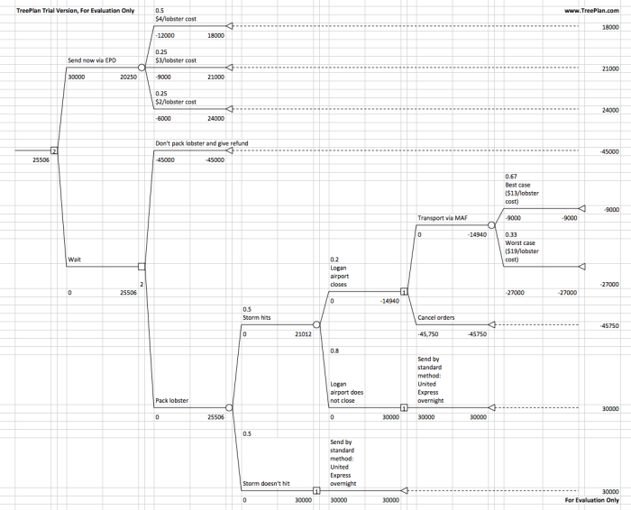
Decision analysis is an important part of modern revenue management strategies for many businesses. One solution for analysis of decisions of smaller complexity is TreePlan, a plugin for Excel. I was required to use TreePlan in an Excel modeling class I took earlier this year to solved the “Kendell Lobster Case” in Bertsimas & Freund’s popular Data, Models, and Decisions.

After solving the case TreePlan’s output looks like this:

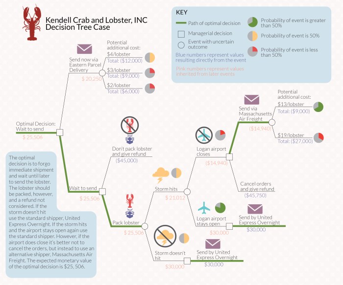
It’s usable, but doesn’t look great. So I took the output and designed a better looking solution using Adobe Illustrator:

Basketball Project Part 4

After researching online basketball data in more depth I found that RealGM had so-called “split” data for college players. Players statistics are sliced in various ways such as performance against Top 25 teams.

n my original collection process involved scraping statistics from every college player, which was quite inefficient. It involved approximately 20,000 player-seasons worth of data and caused problems during the merge since so many players shared names. It also didn’t allow collection of the “split” data since these is housed on each player’s individual page instead of on the “All College Player Stats” page.

It was quite challenging figuring out how to scrape the RealGM site. The page structure was predictable aside from a unique id number for every player, which I assume comes from some sort of internal database on the RealGM site. These numbers range in length from two to five numerals and there is no way I could find to predict these numbers. For instance, Carmelo Anthony’s player page link is below. His player id is 452.

http://basketball.realgm.com/player/Carmelo-Anthony/NCAA/452/2014/By_Split/
Advanced_Stats/Quality_Of_Opp

After a fair bit of thrashing about I finally came up with the solution to write an R script that would google the first portion of the player’s page link, read the Google page source, search for player’s site address using regular expressions, and then append their id to the rest of the structured web address.

For Carmelo, the script would use the following google search link:

https://www.google.com/search?q=realgm.com/player/Carmelo-Anthony

The specificity of the search ensures that the RealGM link appears on the first page of search results (it was the first result in every test scenario I tried). The script then uses the following regular expression when search the Google search results page source:

realgm.com/player/Carmelo-Anthony/(Summary|News|\u2026)/[0-9]+

A player’s main page is always preceded by the player’s name and then “/Summary/id”, but “/News/id” and “/…/id” also appeared. After it locates and reads this link it’s easy enough to strip out the player id and insert it into the player’s page that links to the advanced college data I was looking for.

library(XML)
library(RCurl)
library(data.table)
 
# Read in players and convert names to proper format 
players.DF <- read.csv(file="~/.../Combined Data/Combined Data 1.csv")
players <- as.character(players.DF$Player)
players <- gsub("\\.","",players)
players <- gsub(" ","-",players)
 
# Initialize dataframes and vectors 
missedPlayers <- NULL
playerLinks <- rep(NA, length(players))
playerLinks <- data.frame(players.DF$Player, playerLinks)
 
# Create link for each player 
for(i in 1:length(players)) {
  url <- paste0('https://www.google.com/search?q=realgm.com/player/',players[i])
  result <- try(content <- getURLContent(url))
  if(class(result) == "try-error") { next; }
  id <- regexpr(paste0("realgm.com/player/", players[i],
  "/(Summary|News|\u2026)","/[0-9]+"),content)
 
  id <- substr(content, id, id + attr(id,"match.length"))
  id <- gsub("[^0-9]+","",id)
  id <- paste0('http://basketball.realgm.com/player/', players[i], '/NCAA/', 
  id,'/2014/By_Split/Advanced_Stats/Quality_Of_Opp')
  playerLinks[i,2] <- id
}
 
setnames(playerLinks, c("players.DF.Player","playerLinks"), c("Players","Links"))

Some sites have started to detect and try to prevent web scraping. On iteration 967 Google began blocking my search requests. However, I simply reran the script the next morning from iteration 967 onward to pickup the missing players.

I then used the fact that a missing id results in a page link with “NCAA//” to search for players that were still missing their ids.

> pickups <- playerLinks[which(grepl("NCAA//",playerLinks[[2]])),]

After examining the players I noticed many of these had apostrophes in their name, which I had forgotten to account for in my original name formatting.

I adjusted my procedure and reran the script to get the pickups.

pickups <- playerLinks[which(grepl("NCAA//",playerLinks[[2]])),]
pickups <- pickups[[1]]
pickups <- gsub("'","",pickups)
pickups <- gsub(" ","-",pickups)
pickupNums <- grep("NCAA//",playerLinks[[2]])
 
for(i in 1:length(pickupNums)) {
  j <- pickupNums[i]
  url <- paste0('https://www.google.ca/search?q=realgm.com/player/',pickups[i])
  result <- try(content <- getURLContent(url))
  if(class(result) == "try-error") { next; }
  id <- regexpr(paste0("realgm.com/player/", pickups[i],
  "/(Summary|News|\u2026)","/[0-9]+"),content)
 
  id <- substr(content, id, id + attr(id,"match.length"))
  id <- gsub("[^0-9]+","",id)
  id <- paste0('http://basketball.realgm.com/player/', pickups[i], 
  '/NCAA/', id,'/2014/By_Split/Advanced_Stats/Quality_Of_Opp')
 
  playerLinks[[j,2]] <- id
}

After rerunning the script three players were still missing ids, so I entered these manually.

playerLinks[[370,2]]  <- "http://basketball.realgm.com/player/Eric-Gordon/NCAA/762/2014/By_Split/Advanced_Stats/Quality_Of_Opp"
playerLinks[[884,2]] <- " http://basketball.realgm.com/player/Randolph-Morris/NCAA/166/2014/By_Split/Advanced_Stats/Quality_Of_Opp"
playerLinks[[1010,2]] <- "http://basketball.realgm.com/player/Slavko-Vranes/NCAA/472/2014/By_Split/Advanced_Stats/Quality_Of_Opp"

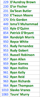
I also needed to manually check the three duplicate players and adjust their ids accordingly.

The final result looks like this:

The next step will be to cycle through the links and use readHTMLTable() to get the advanced statistics.

R Highlighting created by Pretty R at inside-R.org

Basketball Project Part 3

While I was looking around at basketball data during the course of the project I saw that Basketball-Reference.com had a few pieces of data I wanted to pick up: a player’s shooting arm (right or left) and their high school ranking. The site is also packed with a ton of other data I may use in the future such as a player’s shooting percentage from different distances from the basket. So I thought it would be good to create a procedure to scrape it.

The site use a particular website address structure that makes it easy to scrape: http://www.basketball-reference.com/players + the first letter of the player’s last name + the first 5 letters of the player’s last name (unless the player’s name is less than 5 letters in which case their whole name is used + the first two letters of their first name + a page number (usually a 1, but sometimes a 2 if more than one player share a name). For instance, http://www.basketball-reference.com/players/a/anthoca01.html.

R reads the page source and again the site uses a structured page profile:

I first used grep to locate the line of the page source that contained “Shoots:” and “Recruiting Rank:.” And then used regular expressions to strip the information out. Not all players have both (or either) set of information so I used a try() wrapper so the code could practice through errors resulting from no match to the regular expressions.

library(stringr)
 
# Read in master player list
players.DF <- read.csv(file="~/.../All Drafted Players 2013-2003.csv")
allPlayers <- players.DF[,3]
 
# Convert names to proper format
allPlayers <- str_replace_all(allPlayers, "[[:punct:]]", "")
allPlayers <- tolower(allPlayers)
first <- str_extract(allPlayers,"^[^ ]+")
first <- substring(first,1,2)
last <- str_extract(allPlayers,"[^ ]+$")
last <- substring(last,1,5)
letter <- substring(last,1,1)
 
shootsVector <- rep(NA,length(allPlayers))
recruitVector <- rep(NA,length(allPlayers))
 
# Scrape the site and record shooting arm and HSranking
for(i in 1:20) {
  page <- read.csv(paste0(
  'http://www.basketball-reference.com/players/',letter[i],'/',last[i],first[i],'01.html'))
 
  line <- grep("[Ss]hoots:(.*)Right|Left", page[,], value = FALSE, perl = TRUE)
  index <- regexpr("[Rr]ight|[Ll]eft",page[line,])
  shoots <- substr(page[line,], index, index + attr(index,"match.length") - 1)
  result <- try(shootsVector[i] <- shoots)
  if(class(result) == "try-error") { next; }
 
  line <- grep("Recruiting Rank:(.*)([0-9]+)", page[,], value = FALSE, perl = TRUE)
  index <- regexpr("\\([0-9]+\\)$",page[line,])
  recruit <- substr(page[line,], index + 1, index + attr(index,"match.length") - 2)
  result <- try(recruitVector[i] <- recruit)
  if(class(result) == "try-error") { next; }
 
  print(shoots)
  print(recruit)
}
 
# Combine information
players.DF <- cbind(players.DF, shootsVector,recruitVector)
setnames(players.DF,c("shootsVector","recruitVector"),c("Shooting Arm","HS Ranking"))
write.csv(players.DF,file="~/...Combined Data/Combined Data 1.csv")

The procedure is vulnerable to duplicates. There are ways to deal with it in code. One way would be to also read the college from the page source and use that to pick out the player. In this case, however, after running a duplicates report only 3 duplicates were found.

> which(duplicated(allPlayers))
[1]  715  732 1118
> allPlayers[715]
[1] "tony mitchell"
> allPlayers[732]
[1] "chris wright"
> allPlayers[1118]
[1] "jamar smith"

For that reason, it was much easier to just do a manual search on the 6 players and update their data. I choose to do this in Excel. Using the highlight duplicates feature, I could easily scroll down and find the 3 duplicate players and change their shooting arm and HS ranking as necessary.

R Highlighting created by Pretty R at inside-R.org

Basketball Project Part 2

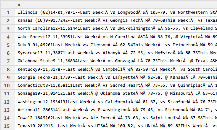
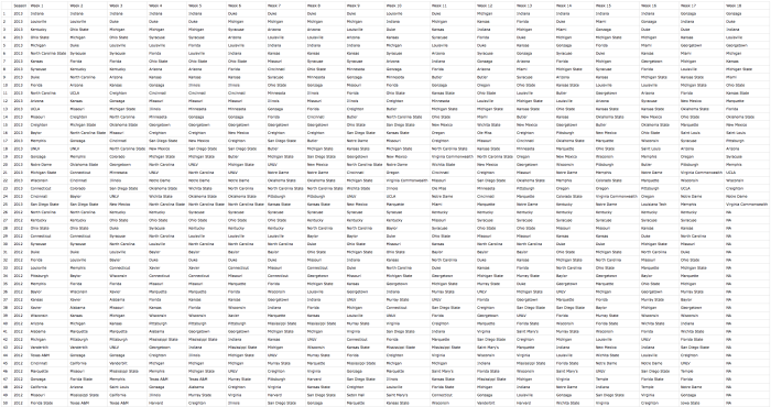
One piece of data I wanted to have for my statistical analysis was the quality of college a player attended. I chose to measure college quality by the number of weeks a team was in the Associated Press (AP) Top 25 college basketball rankings. Note, that I only used regular season rankings not pre- or post-season rankings, which are not available for all years. Historic rankings dating back to the 2002-2003 season are available on the ESPN website. However, when scraping ESPN’s webpage I found the data was semi-structured.

The code to read in the college name must be robust enough to ignore all the possible characters following the college name, but flexible enough to detect “exotic” college names like “Texas A&M” and “St. John’s.” The code first reads in each week’s rankings and strips out the college name. It then binds the weeks together. If the season has less than 18 weeks NAs are introduced to ensure every season is the same length and can be bound together. The college quality is then calculated for each season. Finally, the weekly rankings for every season are bound together into a single table and saved as is the college quality for every season. The code is shown below.

library(XML)
library(data.table)
 
# Initialize variables
seasons <- seq(2013,2003,by=-1)
allSeasonRankings <- NULL
allSeasonTable <- NULL
missedPages <- matrix(ncol=2,nrow=1)
colnames(missedPages) <- c("Season","Week")
k <- 1
 
# Web scrape
# Iterate over each week in each season
for(j in 1:length(seasons)) {
numWeeks <- 0
seasonRanking <- NULL
week <- NULL
 
  for (i in 2:19)
  {
    result <- try(week <- readHTMLTable(paste0(
    'http://espn.go.com/mens-college-basketball/rankings/_/poll/1/year/',
    seasons[j], '/week/', i ,'/seasontype/2'),skip.rows=c(1,2))[[1]][,2])
 
    if(class(result) == "try-error") { missedPages[k,] <- c(j,i); k <- k + 1; next; }
    print(paste0('http://espn.go.com/mens-college-basketball/rankings/_/poll/1/year/', 
    seasons[j], '/week/', i ,'/seasontype/2'))
 
    numWeeks <- numWeeks + 1
    week <- as.data.frame(array(BegString(week)))
    seasonRanking <- cbind(seasonRanking,week[[1]])
    colnames(seasonRanking)[numWeeks] <- paste("Week",numWeeks)   
  }
    # Ensure that all seasons have 18 weeks 
    # (the maximum number of weeks in a season since 2003)
    # so that all seasons have the same length and can easily be bound together
    while(numWeeks < 18) {
      numWeeks <- numWeeks + 1
      extra <- rep(NA,25)
      seasonRanking <- cbind(seasonRanking,extra)
      colnames(seasonRanking)[numWeeks]  <- paste("Week",numWeeks)  
    }
 
# Bind seasons together
allSeasonRankings <- rbind(allSeasonRankings, seasonRanking)
 
# Calculate the percentage of weeks each school was in the AP Top 25
seasonTable <- as.data.frame(table(unlist(seasonRanking)))
percentages <- round((seasonTable[2]/numWeeks)*100,2)
 
# Change column name to "Top 25 %" immediately. Otherwise percentages will 
# inherit the name "Freq" from the table function and not allow use of setnames() 
# since 2 columns have the same name
colnames(percentages)[1] <- "Top 25 %" 
seasonTable <- cbind(seasonTable, percentages)
seasonTable <- cbind(seasonTable, rep(seasons[j],length(seasonTable[1])))
allSeasonTable <- rbind(allSeasonTable,seasonTable)
}
 
# Clean up names
setnames(allSeasonTable,c("Var1", "rep(seasons[j], length(seasonTable[1]))"),
c("Team", "Season"))
 
# Add column with season
rankingYear <- rep(seasons, each=25)
 
# Combine data and cleanup names
allSeasonRankings <- cbind(rankingYear,allSeasonRankings)
allSeasonRankings <- as.data.frame(allSeasonRankings)
setnames(allSeasonRankings,"rankingYear", "Season")
 
# Save files
write.csv(allSeasonRankings,file="~/.../College Quality/Season Rankings.csv")
write.csv(allSeasonTable,file="~/.../College Quality/Percent Time in Top 25.csv")

The above code uses two custom functions to strip out the college name. One, strips out the college name and the second removes the trailing whitespace that sometimes occurs. There are a lot of different ways to do this. The most efficient is probably to use the functionality of the stringr package (such as string_extract()), but I wrote these functions when I was less aware of all of stringr’s functionality.

# Returns first string containing only letters, spaces, and the ' and & symbols
BegString <- function(x) {
  exp <- regexpr("^[a-zA-Z| |.|'|&]+",x)
  stringList <- substr(x,1,attr(exp,"match.length"))
  stringList <- removeTrailSpace(stringList)
  return(stringList)
}

# Removes trailing whitespace of a string
removeTrailSpace <- function(stringList) {
 
  whiteSpaceIndex <- regexpr(" +$",stringList)
  whiteSpaceSize <- attr(whiteSpaceIndex,"match.length")
 
  for(k in 1:length(stringList)) {
    if(whiteSpaceSize[k] > 0) {
      stringList[k] <- substr(stringList[k],1,whiteSpaceIndex[k]-1)
    }
  }
  stringList
}

The weekly ranking table ends up looking like this:

This table is saved purely for reference since all of the meat is in the college quality calculation. College quality is shown below. Again, I kept the “Freq” in for reference so that I could randomly verify the results of a few observations to make sure the code worked properly. As you can see, 43 different teams spent at least one week in the AP Top 25 rankings during 2013.

Now that I have this data I can merge it with the master list of players using the school name and season as keys.

R highlighting created by Pretty R at inside-R.org

Steepest Decent Algorithm

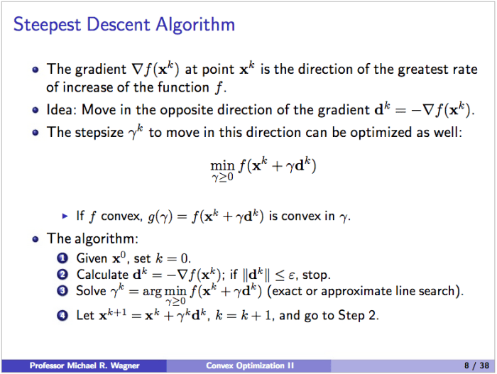
As a homework assignment in a PhD quantitative methods course I took for fun this past quarter – which turned out to be very difficult – we were asked to implement the steepest decent algorithm. This algorithm provides a numeric method to find the minimum of an unconstrained optimization problem. I choose to implement the algorithm in R.

The idea of the algorithm is the following:

Given a particular function it is possible to find a closed form expression for gamma by simply taking the derivative and setting it equal to zero. We were meant only to solve the algorithm for a specific function and associated gamma, but I wrote a more robust R function. It takes an generic function and gamma, an initial location on the function to start the decent, and an epsilon to use as a stopping condition (by changing epsilon we can get an arbitrarily accurate solution).

steepestDecent <- function(x.initial, func = NULL, gamma = NULL, epsilon) {
  # Implement error handling
  if(is.null(func) || is.null(gamma)) { 
    stop("Error: Please enter both a function and gamma.")
  }
 
  require(numDeriv)
  xk <- x.initial
  k <- 1
  xk.vector <- data.frame(k,func(xk))
 
  result <- try(dk <- (-1)*grad(func,xk))
  if(class(result) == "try-error") {
    stop("Error: Make sure dimensions of function and x.star match.")
  }
 
  dk.norm <- norm(dk,'2')
  if(dk.norm <= epsilon) {
    message(sprintf(paste(
      "Error: Starting location is within epsilon tolerance.", 
      "Function value at (%s,%s) is %s.", 
      "Direction norm is %s.", sep=" "),
      xk[1],xk[2],func(xk),dk.norm))
    stop
  }
 
  while(dk.norm > epsilon) {
    dk <- (-1)*grad(func,xk)
    dk.norm <- norm(dk,'2')
    gamma <- gamma(xk,dk)
    xk <- xk + gamma*dk
    k <- k + 1
    current.value <- data.frame(k,func(xk))
    xk.vector <- rbind(xk.vector,current.value)
  }
  ratio.vector <- NULL
  index <- NULL
  func.x.star <- func(xk)
 
  for(i in 1:(length(xk.vector[[1]]) - 1)) {
    try(ratio.vector <- rbind(ratio.vector,((xk.vector[[i+1,2]] - func.x.star)/
    (xk.vector[[i,2]] - func.x.star))))
    if(class(result) == "try-error") {stop}
    index <- rbind(index,i)
  }
  ratio.plot <- plot(index[,1] + 1,ratio.vector[,1],
  main="A Plot of Convergence Ratio vs. K",
  xlab="K",
  ylab="Convergence Ratio")
 
  func.plot <- plot(xk.vector$k,xk.vector$func.xk.,
  main="A plot of f(x^k) as a function of k",
  xlab="K Values",
  ylab="Function Values")
 
  numeric.solution <- sprintf(
  "The numerical approximation of the unconstrained minimum for this function is %s, %s.",
  round(xk[1]), round(xk[2]))
 
  print(xk.vector)
  return(numeric.solution)
}

The function and gamma can be defined separately depending on the problem. We were told to use the following function and gamma:

func <- function(x) {
  x1 <- x[1]
  x2 <- x[2]
  result <- .5*x1^2 - 15*x1 - 5*x1*x2 + 50*x2^2 + 150*x2
  return(result)
}

# Create gamma function
gamma <- function(x,d) {
  x1 <- x[1]
  x2 <- x[2]
  d1 <- d[1]
  d2 <- d[2]
  result <- (-x1*d1 + 5*d1*x2 + 15*d1 + 5*d2*x1 - 100*d2*x2 - 150*d2)/
  (d1**2-10*d1*d2+100*d2**2)
  return(result)
}

My output for the given function and gamma are shown below:

> x.initial <- c(0,0)
> epsilon <- .01
> steepestDecent(x.initial,func,gamma,epsilon)
[1] "The numerical approximation of the unconstrained minimum for this function is 10, -1."

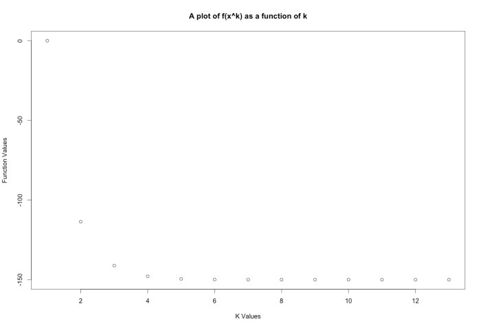
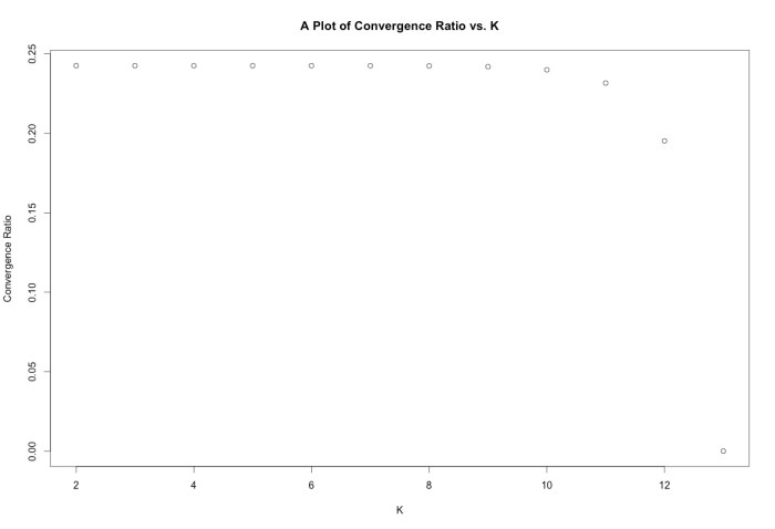
You can see the numerical solution matches the analytical solution found by the standard partial derivative method. The R function also outputs a plot of f(x) as a function of the iteration number as well as a plot of the convergence ratio, given by:

The plots for this function are shown below:

For fun I also created a simple function that uses the necessary and sufficient conditions to check if an x* derived from analytical procedures is a global minimum. The first condition to be a global minimum is that the gradient must be equal to zero. The second fact is that the Hessian matrix of a convex function must be positive semidefinite for all x.

However, if the Hessian can only be verified to be positive semidefinite for a ball of diameter 2*epsilon centered around a given x*, we can only be certain that x* is a local minimum.

On the other hand if the Hessian is not positive semidefinite we aren’t sure of much since we don’t know anything about the shape of the function. Finally, if the gradient is not zero we know for certain that we are not at a minimum since there is some direction we can travel that will lead to a lower f(x).

analyticTest <- function(func, x.star, convex = FALSE) {
  require(numDeriv)
 
  result <- try(hess <- hessian(func,x.star))
  if(class(result) == "try-error") {
    stop("Error: Make sure dimensions of function and x.star match.")
  }  
 
  result <- try(grad <- round(grad(func,x.star),5))
  if(class(result) == "try-error") {
    stop("Error: Make sure dimensions of function and x.star match.")
  }  
 
  if(!isTRUE(all(eigen(hess)[[1]]>0))) {
    print("Hessian matrix not semi-definite. x* not a local or global minimum.")
    print(1)
    return(FALSE)
    }
 
  else if(!isTRUE(all(grad == 0))) {
    print("Gradient at x star is not zero. x* not a local or global minimum.")
    print(2)
    return(FALSE)
    }
 
  else if(convex == TRUE) {
    print("x* is a global minimum.")
    print(3)
    return(TRUE)
    }
 
  else {
    print("x* may be a local or global minimum. Check convexity of function.")
    print(4)
    return(FALSE)
  }    
}

Created by Pretty R at inside-R.org

Thesis Introduction

This is the introduction of my thesis, which was laid out using Adobe InDesign. The chapter header and graphs were created in Illustrator and imported into InDesign.

Tanzania Seed Map

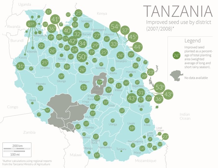
This is a map I created for my thesis on agriculture in Tanzania. The data shows the district variation in the area planted to modern seed varieties. The data is from a 2007-2008 agriculture survey conducted by the Ministry of Agriculture. I used an average of the area planted during the long and short rainy season weighted to account for the fact that most agricultural activity takes place during the long season.