After researching online basketball data in more depth I found that RealGM had so-called “split” data for college players. Players statistics are sliced in various ways such as performance against Top 25 teams.

n my original collection process involved scraping statistics from every college player, which was quite inefficient. It involved approximately 20,000 player-seasons worth of data and caused problems during the merge since so many players shared names. It also didn’t allow collection of the “split” data since these is housed on each player’s individual page instead of on the “All College Player Stats” page.

It was quite challenging figuring out how to scrape the RealGM site. The page structure was predictable aside from a unique id number for every player, which I assume comes from some sort of internal database on the RealGM site. These numbers range in length from two to five numerals and there is no way I could find to predict these numbers. For instance, Carmelo Anthony’s player page link is below. His player id is 452.

http://basketball.realgm.com/player/Carmelo-Anthony/NCAA/452/2014/By_Split/
Advanced_Stats/Quality_Of_Opp

After a fair bit of thrashing about I finally came up with the solution to write an R script that would google the first portion of the player’s page link, read the Google page source, search for player’s site address using regular expressions, and then append their id to the rest of the structured web address.

For Carmelo, the script would use the following google search link:

https://www.google.com/search?q=realgm.com/player/Carmelo-Anthony

The specificity of the search ensures that the RealGM link appears on the first page of search results (it was the first result in every test scenario I tried). The script then uses the following regular expression when search the Google search results page source:

realgm.com/player/Carmelo-Anthony/(Summary|News|\u2026)/[0-9]+

library(XML)
library(RCurl)
library(data.table)
 
# Read in players and convert names to proper format 
players.DF <- read.csv(file="~/.../Combined Data/Combined Data 1.csv")
players <- as.character(players.DF$Player)
players <- gsub("\\.","",players)
players <- gsub(" ","-",players)
 
# Initialize dataframes and vectors 
missedPlayers <- NULL
playerLinks <- rep(NA, length(players))
playerLinks <- data.frame(players.DF$Player, playerLinks)
 
# Create link for each player 
for(i in 1:length(players)) {
  url <- paste0('https://www.google.com/search?q=realgm.com/player/',players[i])
  result <- try(content <- getURLContent(url))
  if(class(result) == "try-error") { next; }
  id <- regexpr(paste0("realgm.com/player/", players[i],
  "/(Summary|News|\u2026)","/[0-9]+"),content)
 
  id <- substr(content, id, id + attr(id,"match.length"))
  id <- gsub("[^0-9]+","",id)
  id <- paste0('http://basketball.realgm.com/player/', players[i], '/NCAA/', 
  id,'/2014/By_Split/Advanced_Stats/Quality_Of_Opp')
  playerLinks[i,2] <- id
}
 
setnames(playerLinks, c("players.DF.Player","playerLinks"), c("Players","Links"))

Some sites have started to detect and try to prevent web scraping. On iteration 967 Google began blocking my search requests. However, I simply reran the script the next morning from iteration 967 onward to pickup the missing players.

I then used the fact that a missing id results in a page link with “NCAA//” to search for players that were still missing their ids.

> pickups <- playerLinks[which(grepl("NCAA//",playerLinks[[2]])),]

I adjusted my procedure and reran the script to get the pickups.

pickups <- playerLinks[which(grepl("NCAA//",playerLinks[[2]])),]
pickups <- pickups[[1]]
pickups <- gsub("'","",pickups)
pickups <- gsub(" ","-",pickups)
pickupNums <- grep("NCAA//",playerLinks[[2]])
 
for(i in 1:length(pickupNums)) {
  j <- pickupNums[i]
  url <- paste0('https://www.google.ca/search?q=realgm.com/player/',pickups[i])
  result <- try(content <- getURLContent(url))
  if(class(result) == "try-error") { next; }
  id <- regexpr(paste0("realgm.com/player/", pickups[i],
  "/(Summary|News|\u2026)","/[0-9]+"),content)
 
  id <- substr(content, id, id + attr(id,"match.length"))
  id <- gsub("[^0-9]+","",id)
  id <- paste0('http://basketball.realgm.com/player/', pickups[i], 
  '/NCAA/', id,'/2014/By_Split/Advanced_Stats/Quality_Of_Opp')
 
  playerLinks[[j,2]] <- id
}

After rerunning the script three players were still missing ids, so I entered these manually.

playerLinks[[370,2]]  <- "http://basketball.realgm.com/player/Eric-Gordon/NCAA/762/2014/By_Split/Advanced_Stats/Quality_Of_Opp"
playerLinks[[884,2]] <- " http://basketball.realgm.com/player/Randolph-Morris/NCAA/166/2014/By_Split/Advanced_Stats/Quality_Of_Opp"
playerLinks[[1010,2]] <- "http://basketball.realgm.com/player/Slavko-Vranes/NCAA/472/2014/By_Split/Advanced_Stats/Quality_Of_Opp"

I also needed to manually check the three duplicate players and adjust their ids accordingly.

The final result looks like this:

The next step will be to cycle through the links and use readHTMLTable() to get the advanced statistics.

R Highlighting created by Pretty R at inside-R.org

While I was looking around at basketball data during the course of the project I saw that Basketball-Reference.com had a few pieces of data I wanted to pick up: a player’s shooting arm (right or left) and their high school ranking. The site is also packed with a ton of other data I may use in the future such as a player’s shooting percentage from different distances from the basket. So I thought it would be good to create a procedure to scrape it.

The site use a particular website address structure that makes it easy to scrape: http://www.basketball-reference.com/players + the first letter of the player’s last name + the first 5 letters of the player’s last name (unless the player’s name is less than 5 letters in which case their whole name is used + the first two letters of their first name + a page number (usually a 1, but sometimes a 2 if more than one player share a name). For instance, http://www.basketball-reference.com/players/a/anthoca01.html.

R reads the page source and again the site uses a structured page profile:

I first used grep to locate the line of the page source that contained “Shoots:” and “Recruiting Rank:.” And then used regular expressions to strip the information out. Not all players have both (or either) set of information so I used a try() wrapper so the code could practice through errors resulting from no match to the regular expressions.

library(stringr)
 
# Read in master player list
players.DF <- read.csv(file="~/.../All Drafted Players 2013-2003.csv")
allPlayers <- players.DF[,3]
 
# Convert names to proper format
allPlayers <- str_replace_all(allPlayers, "[[:punct:]]", "")
allPlayers <- tolower(allPlayers)
first <- str_extract(allPlayers,"^[^ ]+")
first <- substring(first,1,2)
last <- str_extract(allPlayers,"[^ ]+$")
last <- substring(last,1,5)
letter <- substring(last,1,1)
 
shootsVector <- rep(NA,length(allPlayers))
recruitVector <- rep(NA,length(allPlayers))
 
# Scrape the site and record shooting arm and HSranking
for(i in 1:20) {
  page <- read.csv(paste0(
  'http://www.basketball-reference.com/players/',letter[i],'/',last[i],first[i],'01.html'))
 
  line <- grep("[Ss]hoots:(.*)Right|Left", page[,], value = FALSE, perl = TRUE)
  index <- regexpr("[Rr]ight|[Ll]eft",page[line,])
  shoots <- substr(page[line,], index, index + attr(index,"match.length") - 1)
  result <- try(shootsVector[i] <- shoots)
  if(class(result) == "try-error") { next; }
 
  line <- grep("Recruiting Rank:(.*)([0-9]+)", page[,], value = FALSE, perl = TRUE)
  index <- regexpr("\\([0-9]+\\)$",page[line,])
  recruit <- substr(page[line,], index + 1, index + attr(index,"match.length") - 2)
  result <- try(recruitVector[i] <- recruit)
  if(class(result) == "try-error") { next; }
 
  print(shoots)
  print(recruit)
}
 
# Combine information
players.DF <- cbind(players.DF, shootsVector,recruitVector)
setnames(players.DF,c("shootsVector","recruitVector"),c("Shooting Arm","HS Ranking"))
write.csv(players.DF,file="~/...Combined Data/Combined Data 1.csv")

The procedure is vulnerable to duplicates. There are ways to deal with it in code. One way would be to also read the college from the page source and use that to pick out the player. In this case, however, after running a duplicates report only 3 duplicates were found.

> which(duplicated(allPlayers))
[1]  715  732 1118
> allPlayers[715]
[1] "tony mitchell"
> allPlayers[732]
[1] "chris wright"
> allPlayers[1118]
[1] "jamar smith"

For that reason, it was much easier to just do a manual search on the 6 players and update their data. I choose to do this in Excel. Using the highlight duplicates feature, I could easily scroll down and find the 3 duplicate players and change their shooting arm and HS ranking as necessary.

R Highlighting created by Pretty R at inside-R.org

One piece of data I wanted to have for my statistical analysis was the quality of college a player attended. I chose to measure college quality by the number of weeks a team was in the Associated Press (AP) Top 25 college basketball rankings. Note, that I only used regular season rankings not pre- or post-season rankings, which are not available for all years. Historic rankings dating back to the 2002-2003 season are available on the ESPN website. However, when scraping ESPN’s webpage I found the data was semi-structured.

The code to read in the college name must be robust enough to ignore all the possible characters following the college name, but flexible enough to detect “exotic” college names like “Texas A&M” and “St. John’s.” The code first reads in each week’s rankings and strips out the college name. It then binds the weeks together. If the season has less than 18 weeks NAs are introduced to ensure every season is the same length and can be bound together. The college quality is then calculated for each season. Finally, the weekly rankings for every season are bound together into a single table and saved as is the college quality for every season. The code is shown below.

library(XML)
library(data.table)
 
# Initialize variables
seasons <- seq(2013,2003,by=-1)
allSeasonRankings <- NULL
allSeasonTable <- NULL
missedPages <- matrix(ncol=2,nrow=1)
colnames(missedPages) <- c("Season","Week")
k <- 1
 
# Web scrape
# Iterate over each week in each season
for(j in 1:length(seasons)) {
numWeeks <- 0
seasonRanking <- NULL
week <- NULL
 
  for (i in 2:19)
  {
    result <- try(week <- readHTMLTable(paste0(
    'http://espn.go.com/mens-college-basketball/rankings/_/poll/1/year/',
    seasons[j], '/week/', i ,'/seasontype/2'),skip.rows=c(1,2))[[1]][,2])
 
    if(class(result) == "try-error") { missedPages[k,] <- c(j,i); k <- k + 1; next; }
    print(paste0('http://espn.go.com/mens-college-basketball/rankings/_/poll/1/year/', 
    seasons[j], '/week/', i ,'/seasontype/2'))
 
    numWeeks <- numWeeks + 1
    week <- as.data.frame(array(BegString(week)))
    seasonRanking <- cbind(seasonRanking,week[[1]])
    colnames(seasonRanking)[numWeeks] <- paste("Week",numWeeks)   
  }
    # Ensure that all seasons have 18 weeks 
    # (the maximum number of weeks in a season since 2003)
    # so that all seasons have the same length and can easily be bound together
    while(numWeeks < 18) {
      numWeeks <- numWeeks + 1
      extra <- rep(NA,25)
      seasonRanking <- cbind(seasonRanking,extra)
      colnames(seasonRanking)[numWeeks]  <- paste("Week",numWeeks)  
    }
 
# Bind seasons together
allSeasonRankings <- rbind(allSeasonRankings, seasonRanking)
 
# Calculate the percentage of weeks each school was in the AP Top 25
seasonTable <- as.data.frame(table(unlist(seasonRanking)))
percentages <- round((seasonTable[2]/numWeeks)*100,2)
 
# Change column name to "Top 25 %" immediately. Otherwise percentages will 
# inherit the name "Freq" from the table function and not allow use of setnames() 
# since 2 columns have the same name
colnames(percentages)[1] <- "Top 25 %" 
seasonTable <- cbind(seasonTable, percentages)
seasonTable <- cbind(seasonTable, rep(seasons[j],length(seasonTable[1])))
allSeasonTable <- rbind(allSeasonTable,seasonTable)
}
 
# Clean up names
setnames(allSeasonTable,c("Var1", "rep(seasons[j], length(seasonTable[1]))"),
c("Team", "Season"))
 
# Add column with season
rankingYear <- rep(seasons, each=25)
 
# Combine data and cleanup names
allSeasonRankings <- cbind(rankingYear,allSeasonRankings)
allSeasonRankings <- as.data.frame(allSeasonRankings)
setnames(allSeasonRankings,"rankingYear", "Season")
 
# Save files
write.csv(allSeasonRankings,file="~/.../College Quality/Season Rankings.csv")
write.csv(allSeasonTable,file="~/.../College Quality/Percent Time in Top 25.csv")

The above code uses two custom functions to strip out the college name. One, strips out the college name and the second removes the trailing whitespace that sometimes occurs. There are a lot of different ways to do this. The most efficient is probably to use the functionality of the stringr package (such as string_extract()), but I wrote these functions when I was less aware of all of stringr’s functionality.

# Returns first string containing only letters, spaces, and the ' and & symbols
BegString <- function(x) {
  exp <- regexpr("^[a-zA-Z| |.|'|&]+",x)
  stringList <- substr(x,1,attr(exp,"match.length"))
  stringList <- removeTrailSpace(stringList)
  return(stringList)
}

# Removes trailing whitespace of a string
removeTrailSpace <- function(stringList) {
 
  whiteSpaceIndex <- regexpr(" +$",stringList)
  whiteSpaceSize <- attr(whiteSpaceIndex,"match.length")
 
  for(k in 1:length(stringList)) {
    if(whiteSpaceSize[k] > 0) {
      stringList[k] <- substr(stringList[k],1,whiteSpaceIndex[k]-1)
    }
  }
  stringList
}

As part of a graduate applied regression course I took we were required to create and present a research question. The top third of the questions were assigned three students, and these groups worked on the project for the last seven weeks of class. I proposed examining the relationship between early career NBA performance and a variety of pre-NBA player attributes.

NBA performance was to be measured using the co-called “Player Efficiency Rating” created by John Hollinger (usually denoted simply “PER”). The PER attempts to combine all of a player’s on-court statistics into a single number, with the NBA average set to 15 every season. The pre-NBA player profile included a variety of advanced statistics measuring shooting, rebounding, steals, assists, and blocks. For some players NBA combine data was also available. The combine data consisted of a variety of body measurements and results from athletic skills tests (such as standing vertical leap).

My team and I worked throughout the quarter and presented our results last week at the class poster presentation. However, I wanted to redo the project on my own time with better data and full control over the data analysis (rather than having to split up the work between there people).

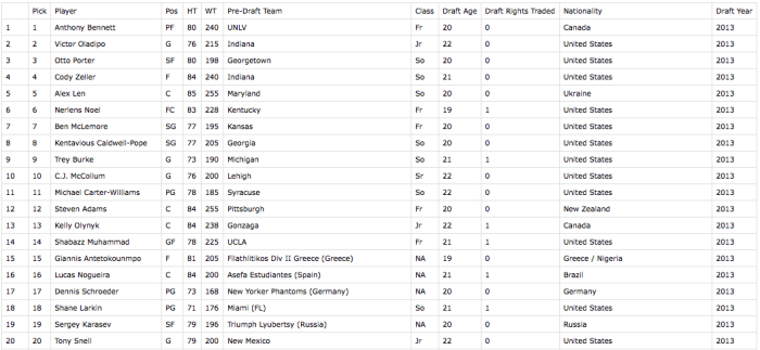
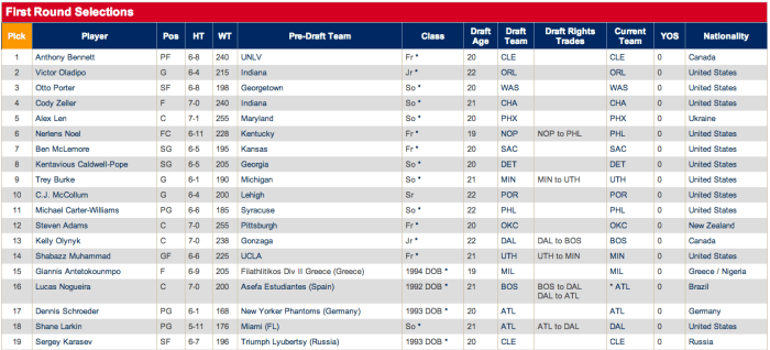
Since this is the second time around I’m much smarter about how to cull, clean, and merge the data efficiently. The first step is to get a master list of players. I’m choosing to use RealGM Basketball’s draft data. It includes both drafted and undrafted players that played in the NBA (or D-league) dating back to 1978. The procedure I used (shown below) works for the modern two-round draft, which started in 1989. However, since college data is only available from the 2002-2003 season, I only went as far back as the 2003 NBA draft.

This dataset includes draft age, an obvious proxy for age a player began his on-court NBA career, something missing from our original dataset. It includes country of birth as well, which would allow a test of the common assertion that foreign players are better shooters. Importantly, this dataset also includes a player’s college name in a format that matches the Associated Press (AP) Top 25 rankings available on ESPN’s website. For instance, depending on the data source the University of Kentucky is sometimes written as “University of Kentucky”, elsewhere simply as “Kentucky”, and occasionally as “UK” (ESPN’s site uses the variant “Kentucky”). I’ve learned that thinking carefully beforehand about how to merge data saves a lot of pain later.

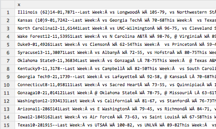
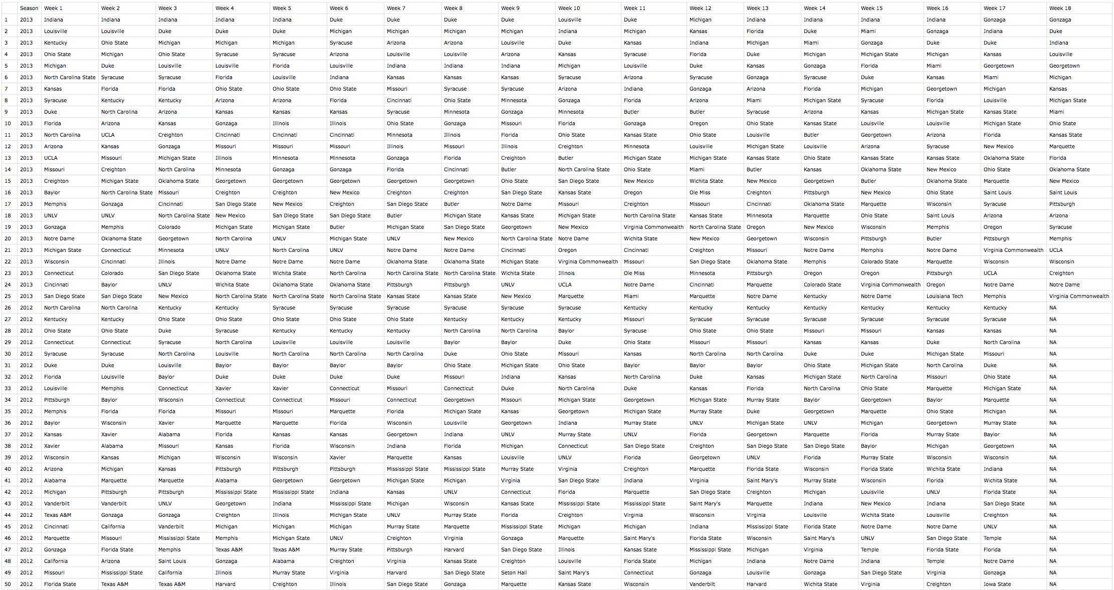
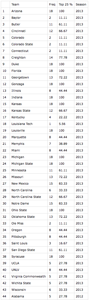
Controlling for the quality of a player’s college basketball program was an unfortunate omission from the original analysis. Because it embodies both the quality of coaching a player received and toughness of competition they faced it may have been a cause of omitted variable bias. For this measure I’ve decided on using the percentage of the season a team was in the AP Top 25 rankings.

To get this master player list I used R’s XML package to scrape the RealGM site. I used try() in conjunction with readHTMLTable() since otherwise my intermittent internet (or other unexpected problems) would cause the for() loop to stop completely. If try() encounters an error I log the page so I can examine it later and pickup any missing data.

After the scrape I examined the data and had to do some simple cleaning. Drafted and undrafted players have slightly different data available so I had to introduce some NA’s for the undrafted players so I could combine the dataframes. I also had to convert the columns from factors to characters or numeric depending on their values. Height, which in its native format as feet-inches (ex. 6-10) needed to be converted to a pure numeric value (I used height in inches). And a few columns had extra characters that needed to be removed.

To convert height I wrote a custom function (shown below). I could have used the R package stringr’s function str_extract() instead of regexpr() and substr(), but for variety (and practice) I went with the less efficient two-line approach.  In general, the length of my code could be substantially reduce, but at the cost of readability for others (as well as myself when I revisit the code in the future).

convertHeight <- function(x) {
  feet <- substr(x,1,1)
  inches <- regexpr("[0-9]+$",x)
  inches <- substr(x, inches, inches + attr(inches,"match.length"))
  height <- as.numeric(feet)*12 + as.numeric(inches)
  return(height)
}

Everything went smoothly aside from a warning that NA’s were introduced by coercion when converting “Weight” to numeric. After a quick search it turns out this was only a problem for a single player, number 1073.

> which(is.na(allPlayers[,5]) == TRUE)
[1] 1073

Player 1073 turns out to be Donell Williams from Fayetteville State who went undrafted in 2005 and later played a season in the D-league. I went back to RealGM’s site and confirmed that his weight was indeed marked as “N/A” in the source data.

The next steps will be to merge in the college quality data (from ESPN), a few additional pieces of data I scraped from Basketball-Reference (such as the shooting hand a player uses), all of the NBA combine data (from DraftExpress), and the players’ college and NBA statistics (from RealGM and Basketball-Reference). Each piece of data requires it’s own web scraping and cleaning, which I’ll take up in future posts.

# Load necessary libraries
library(XML)
library(data.table)
library(stringr)
 
# Initialize variables
round1 <- NULL
round2 <- NULL
drafted <- NULL
undrafted <- NULL
allDraftedPlayers <- NULL
allUndraftedPlayers <- NULL
missedPages <- NULL
seasons <- seq(2013,2003,by=-1)
 
# Get draft info for drafted and undrafted players
for(i in 1:length(seasons))
{                        
    result <- try(page<-readHTMLTable(paste0(
    'http://basketball.realgm.com/nba/draft/past_drafts/', seasons[i])))
    if(class(result) == "try-error") { missedPages <- rbind(missedPages,seasons[i]); next; }
 
    round1 <- page[[3]]
    round2 <- page[[4]]
    drafted <- rbind(round1,round2)
    undrafted <- page[[5]]
 
    # Print data for monitoring
    print(paste0('http://basketball.realgm.com/nba/draft/past_drafts/', seasons[i]))
    print(head(round1))
    print(head(round2))
    print(head(undrafted))
 
    # Add draft year and combine data
    draftYear <- rep(seasons[i], dim(drafted)[1])
    print(head(draftYear))
    drafted <- cbind(drafted,draftYear)
    allDraftedPlayers <- rbind(allDraftedPlayers,drafted)
    draftYear <- rep(seasons[i], dim(undrafted)[1])
    undrafted <- cbind(undrafted,draftYear)
    allUndraftedPlayers <- rbind(allUndraftedPlayers, undrafted)  
}
 
# Drop unused columns
allDraftedPlayers <- allDraftedPlayers[,-c(9,11:12)]
allUndraftedPlayers <- allUndraftedPlayers[,-c(8:9)]
 
# Add NAs to undrafted players as necessary
length <- length(allUndraftedPlayers[[1]])
allUndraftedPlayers <- cbind(rep(NA, length),allUndraftedPlayers[,c(1:7)],rep(NA,length),
allUndraftedPlayers[,c(8:9)])
 
# Unify names so rbind can combine datasets
colnames(allUndraftedPlayers)[1] <- "Pick"
colnames(allUndraftedPlayers)[9] <- "Draft RightsTrades"
allPlayers <- rbind(allDraftedPlayers,allUndraftedPlayers)
 
# Cleanup column names
setnames(allPlayers,c("DraftAge","Draft RightsTrades","draftYear"),
c("Draft Age","Draft Rights Traded","Draft Year"))
 
# Convert columns from factors to character and numeric as necessary
allPlayers[,-3] <- data.frame(lapply(allPlayers[,-3], as.character), 
stringsAsFactors=FALSE)
allPlayers[,c(5,8)] <- data.frame(lapply(allPlayers[,c(5,8)], as.numeric), 
stringsAsFactors=FALSE)
 
# Add dummy if player was traded on draft day
traded <- allPlayers[[9]]
allPlayers[which(regexpr("[a-zA-Z]+",traded) != -1), 9] <- 1
allPlayers[which(allPlayers[[9]] != 1), 9] <- 0
 
# Get rid of extra characters in class (mostly astricks)
allPlayers[[7]] <- str_extract(allPlayers[[7]],"[a-zA-Z]+")
allPlayers[[7]] <- gsub("DOB",NA,allPlayers[[7]])
 
# Convert height to inches from feet-inches format
allPlayers[[4]] <- convertHeight(allPlayers[[4]])
 
# Function for converting height
convertHeight <- function(x) {
  feet <- substr(x,1,1)
  inches <- regexpr("[0-9]+$",x)
  inches <- substr(x, inches, inches + attr(inches,"match.length"))
  height <- as.numeric(feet)*12 + as.numeric(inches)
  return(height)
}
 
write.csv(allPlayers,file="~/.../Draft Info/All Drafted Players 2013-2003.csv")

R Highlighting created by Pretty R at inside-R.org

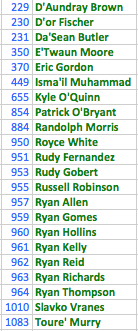
The result is to take this:

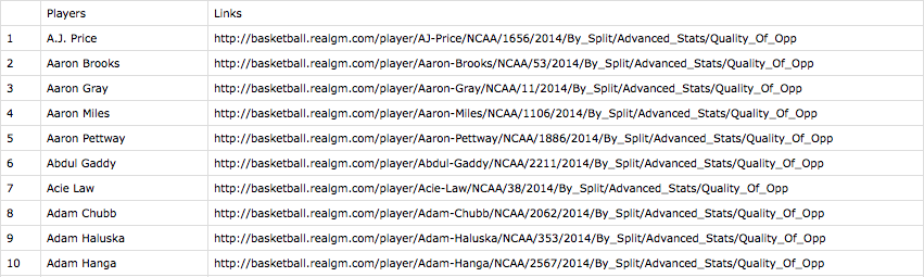
And transform it into this: