
I decided I wanted to get better at geography and I found some quizzes online to help me practice. After a few weeks of practice I’m now able to find the location of every country on earth (video screen capture). Next up: (1) capitols (2) being able to draw and the location of every country from scratch with it’s rough shape, correct bordering countries, and correct country spelling. Then I’m going to memorize other important geographic entities such as lakes, rivers, and mountains. With my current plan I should be finished by the end of this year.
Category: Uncategorized
One-Sentence Summaries
1. Steve Jobs by Walter Isaacson
Intuition > Data; cry as much as you want; demand the best out of people.
2. Kitchen Confidential: Adventures in the Culinary Underbelly by Anthony Bourdain
America’s best restaurants rely on a pro-Ecuadorian immigration policy.
3. What Is Strategy? by Michael E. Porter (C. Roland Christensen Professor of Business Administration, Harvard Business School)
Don’t do things better, anyone can do that; do things differently.
4. Paddington
Wes Anderson meets Being There with a sprinkling of The Adventures of Tin Tin guest starring Cruella de Vil as Ethan Hunt. Plus a bear.
5. The Boys in the Boat: Nine Americans and Their Epic Quest for Gold at the 1936 Berlin Olympics by Daniel James Brown
Mind in boat.
6. Malcolm X: The Last Speeches by Malcolm X
Militancy in a time America was militant.
7. Into Thin Air by Jon Krakauer
Socialization can make you a killer.
8. Seattle Children’s Theatre’s Robin Hood.
Kids love when grown men get hit in the butt with swords.
9. American Snipper by Chris Kyle
War vignettes.
What I’m Reading
Just finished:
1. Steve Jobs by Walter Isaacson
2. Kitchen Confidential: Adventures in the Culinary Underbelly by Anthony Bourdain
3. What Is Strategy? by Michael E. Porter (C. Roland Christensen Professor of Business Administration, Harvard Business School)
Up next:
The Boys in the Boat: Nine Americans and Their Epic Quest for Gold at the 1936 Berlin Olympics by Daniel James Brown
In the queue:
1. American Sniper: The Autobiography of the Most Lethal Sniper in U.S. Military History by Chris Kyle, Scott McEwan, Jim DeFelice
2. A Short History of Nearly Everything by Bill Bryson
3. A Passage to India by E. M. Forster
4. Classic Love Poems by William Shakespeare, Edgar Allan Poe, Elizabeth Barrett Browning
5. How Google Works by Eric Schmidt, Jonathan Rosenberg, Alan Eagle
6. Fahrenheit 451 by Ray Bradbury
7. Warren Buffett and the Interpretation of Financial Statements: The Search for the Company with a Durable Competitive Advantage by Mary Buffett, David Clark
8. How to Read and Understand Shakespeare by The Great Courses
9. Into Thin Air by Jon Krakauer
10. Malcolm X: The Last Speeches by Malcolm X
11. Cary Grant Radio Movies Collection by Lux Radio Theatre, Screen Director’s Playhouse
12. Murder on the Orient Express: A Hercule Poirot Mystery by Agatha Christie
13. Age of Ambition: Chasing Fortune, Truth, and Faith in the New China by Evan Osnos
14. Race Matters by Cornel West
15. The Everything Store: Jeff Bezos and the Age of Amazon by Brad Stone
Creating “Tidy” Web Traffic Data in R
There are many tutorials for transforming data using R, but I wanted to demonstrate how you might create dummy web traffic data and then make it tidy ( have one row for every observation) so that it can be further processed using statistical modeling.
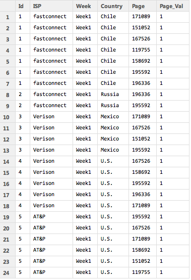
The sample data I created looks like the table below. So there is a separate line for each ID. This might be a visitor ID or a session ID. The ISP, week, and country are the same for every row of the ID. But the page ID is different. If the user visited five different pages they would have five unique rows. Two pages, two rows. And so on. You can imagine many different scenarios where you might have a dataset structured in this way. The column “Page_Val” is a custom column that must be added to the dataset by the user. When we pivot the data each page ID will become it’s own column. If a user visited a particular page Page-Val will be used to add a 1 to that page ID column for that user. Otherwise an NA will appear. We can then go back and replace all the NAs with 0s. I used two lines of code to perform the transformation and replacing of NAs with 0s, but using the fill parameter in the dcast function in “reshape2” it can actually be done in a single line. That’s why it pays to read the documentation very closely, which I didn’t do the first time around. Shame on me.
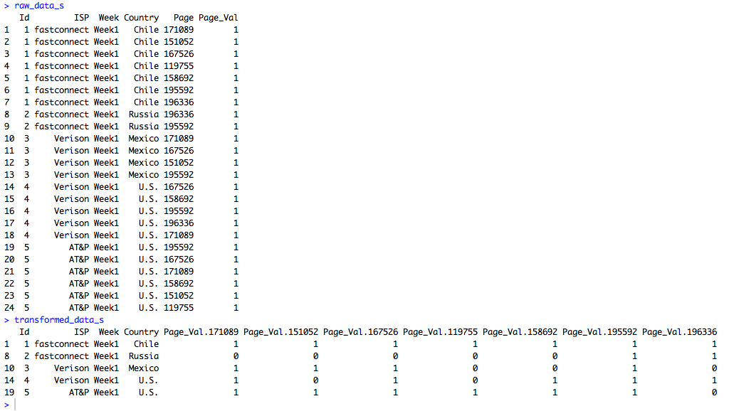
Because the sample data is so small the data can easily be printed out to the screen before and after the transformation.
But the data doesn’t have to be small. In fact, I wrote a custom R function that generates this dummy data. It can easily produce large amounts of dummy data so more robust excercises can be performed. For instance, I produced 1.5 million rows of data in just a couple of seconds and then ran speed tests using the standard reshape function in one trial and the dcast function from “reshape2” in another trial. The dcast function was about 15 times faster in transforming the data. All of the R code is below.
###############################################################################################
# James McCammon
# Wed, 18 March 2015
#
# File Description:
# This file demonstrates how to transform dummy website data from long to wide format.
# The dummy data is strucutred so that there are mulitple rows for each visit, with
# each visit row containing a unique page id representing a different webpage viewed
# in that visit. The goal is to transform the data so that each visit is a single row,
# with webpage ids transformed into columns names with 1s and 0s as values representing
# whether  the page was viewed in that particular visit. This file demonstrates two different
# methods to accomplish this task. It also performs a speed test to determine which
# of the two methods is faster.
###############################################################################################

# Install packages if necessary
needed_packages = c("reshape2", "norm")
new_packages = needed_packages[!(needed_packages %in% installed.packages()[,"Package"])]
if(length(new_packages)) install.packages(new.packages)

###############################################################################################
# Create small amount of raw dummy data
###############################################################################################
# Make a function to create dummy data
get_raw_data = function(num_visitors, n, ids, isps, weeks, countries, pages) {
  raw_data = cbind.data.frame(
    'Id' = do.call(rep, list(x=ids, times=n)),
    'ISP' = isps[do.call(rep, list(x=sample(1:length(isps), size=num_visitors, replace=TRUE), times=n))],
    'Week' = weeks[do.call(rep, list(x=sample(1:length(weeks), size=num_visitors, replace=TRUE), times=n))],
    'Country' = countries[do.call(rep, list(x=sample(1:length(countries), size=num_visitors, replace=TRUE), times=n))],
    'Page' = unlist(sapply(n, FUN=function(i) sample(pages, i))),
    'Page_Val' = rep(1, times=sum(n)))
  raw_data
}

# Set sample parameters to draw from when creating dummy raw data
num_visitors = 5
max_row_size = 7
ids = 1:num_visitors
isps = c('Digiserve', 'Combad', 'AT&P', 'Verison', 'Broadserv', 'fastconnect')
weeks = c('Week1')
countries = c('U.S.', 'Brazil', 'China', 'Canada', 'Mexico', 'Chile', 'Russia')
pages = as.character(sample(100000:200000, size=max_row_size, replace=FALSE))
n = sample(1:max_row_size, size=num_visitors, replace=TRUE)
# Create a small amount of dummy raw data
raw_data_s = get_raw_data(num_visitors, n, ids, isps, weeks, countries, pages)

###############################################################################################
# Transform raw data: Method 1
###############################################################################################
# Reshape data
transformed_data_s = reshape(raw_data_s,
                timevar = 'Page',
                idvar = c('Id', 'ISP', 'Week', 'Country'),
                direction='wide')
# Replace NAs with 0
transformed_data_s[is.na(transformed_data_s)] = 0

# View the raw and transformed versions of the data
raw_data_s
transformed_data_s

###############################################################################################
# Transform raw data: Method 2
###############################################################################################
# Load libraries
require(reshape2)
require(norm)

# Transform the data using dcast from the reshape2 package
transformed_data_s = dcast(raw_data_s, Id + ISP + Week + Country ~ Page, value.var='Page_Val')
# Replace NAs using a coding function from the norm package
transformed_data_s = .na.to.snglcode(transformed_data_s, 0)
# An even simpler way of filling in missing data with 0s is to
# specify fill=0 as an argument to dcast.

# View the raw and transformed versions of the data
raw_data_s
transformed_data_s

###############################################################################################
# Run speed tests on larger data
###############################################################################################
# Caution: This will create a large data object and run several functions that may take a
# while to run on your machine. As a cheat sheet the results of the test are as follows:
# The transformation method that used the standard "reshape" command took 28.3 seconds
# The transformation method that used "dcast" from the "reshape2" package took 1.8 seconds

# Set sample parameters to draw from when creating dummy raw data
num_visitors = 100000
max_row_size = 30
ids = 1:num_visitors
pages = as.character(sample(100000:200000, size=max_row_size, replace=FALSE))
n = sample(1:max_row_size, size=num_visitors, replace=TRUE)
# Create a large amount of raw dummy data
raw_data_l = get_raw_data(num_visitors, n, ids, isps, weeks, countries, pages)

s1 = system.time({
  transformed_data_l = reshape(raw_data_l,
                               timevar = 'Page',
                               idvar = c('Id', 'ISP', 'Week', 'Country'),
                               direction='wide')
  transformed_data_l[is.na(transformed_data_l)] = 0
})

s2 = system.time({
  transformed_data_l = dcast(raw_data_l, Id + ISP + Week + Country ~ Page, value.var='Page_Val')
  transformed_data_l = .na.to.snglcode(transformed_data_l, 0)
})

s1[3]
s2[3]
More Access Tricks
Using the student data files from Pearson Higher Education that go along with the GO! Microsoft Access book. Conditional queries:  Using Is Null to find missing data:
  Using sum to find total scholarship funds by department.
  Using crosstabs:
 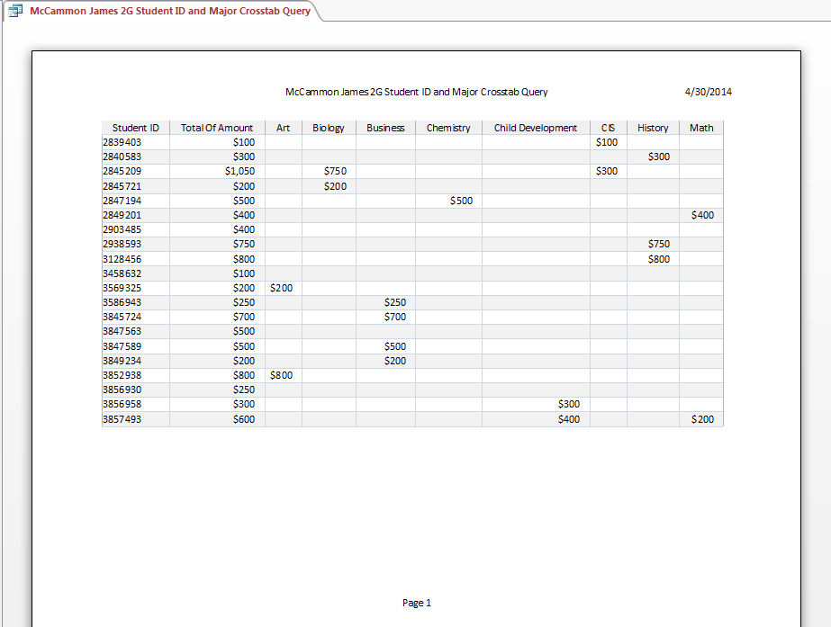 Requiring a major be entered to complete the search.
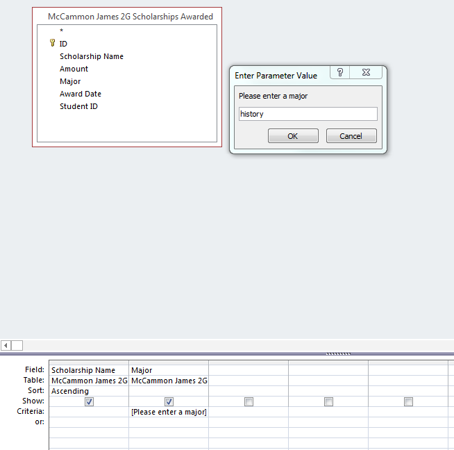
LaTeX in WordPress
As part of a recent post on ridge and lasso regression techniques in R I wanted to present two mathamatical formulas. I checked for WordPress plugins that used LaTeX, but I learned you have to migrate your blog from WordPress.com to WordPress.org and I didn’t want to have to deal with that. Turns out I don’t have to! WordPress itself supports many of the features of LaTeX. You simple write “$latex” before your math equation, use standard LaTeX syntax, and then close with another “$”. Just like in LaTeX itself!! Below are two example equations I presented in my post:
Ridge Regression:

Lasso Regression:

Microsoft Access
I’m learning Microsoft Access as part of a class from UW’s Information School. A lot of people are down on Microsoft, but in my opinion they usually do a good job with Office products. Access is pretty easy to learn and use and it seems powerful. It’s actually a great way to organize information even if you aren’t going to use much of the database functionality. I put some of the World Bank LSMS data I’ve been analyzing for my thesis and it’s a great way to visualize the linkages. The World Bank data has over 30 files with various one-to-one, many-to-one, and one-to-many relationships and Access seems like it would be a good platform to get a handle on the data. Although you can’ t do hardcore data analysis with Access, I think for simple data exploration using reports, queries, and forms could be quite useful.
Below are a couple of screenshots of some of the project assignments we’ve had that simulate a community college administration office.


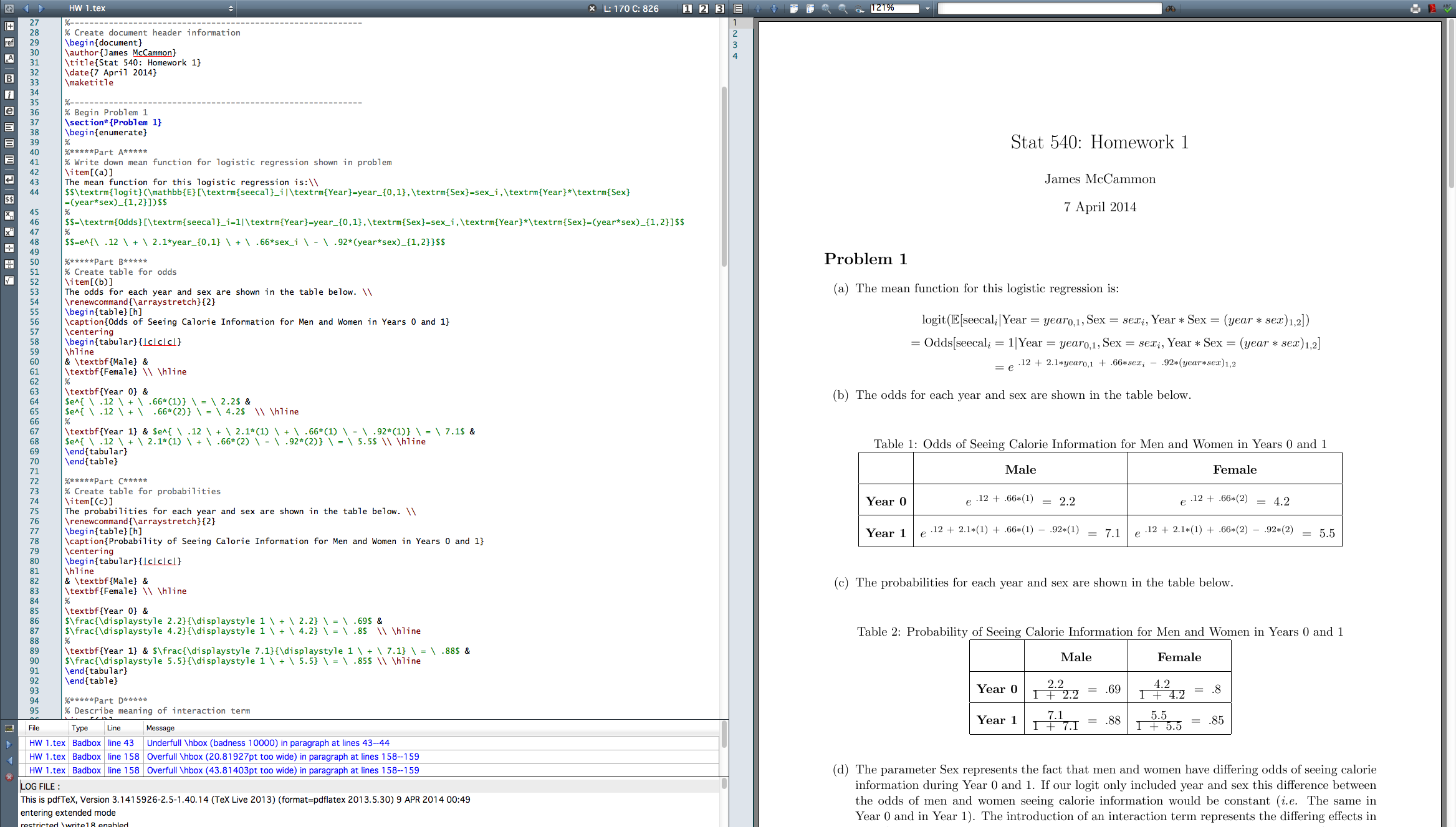
I Finally Learned LaTeX!
I finally got around to learning LaTeX last night, which is a document preparation system for math and statistics papers. The best way I know how to describe it is like HTML, but for documents. It’s much easier to learn and use than HTML, but does have a particular syntax to make text bold, add section headers, and so on. Here’s a screenshot to give a feel of the interface (I use TexMaker). The code on the left produces the PDF on the right.
LaTeX documents have a very distinctive look. You may recognize the format if you’ve taken a math class in college because many professors write their assignments using it.
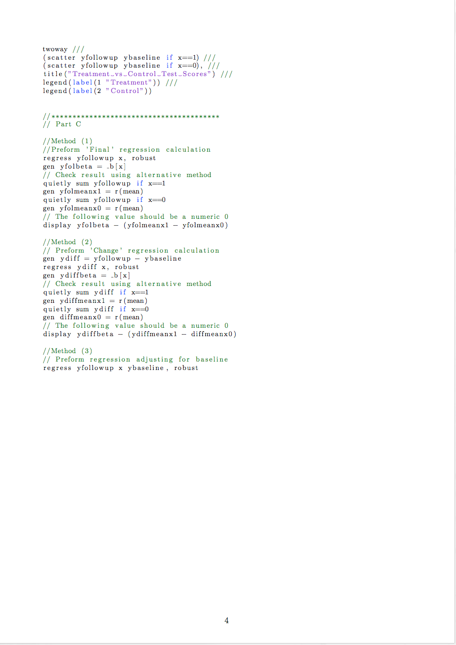
I was even able to find that the listings package does syntax highlighting. Unfortunately, Stata is not supported. I played around with telling LaTeX that I was using Python, Java, etc. until the highlighting rules for that language matched somewhat with the way Stata should be highlighted. Java was the best match I found. There is also a package called minted, but it requires a little more work for installation and I didn’t have the time to mess around with it. I’m not even sure if it supports Stata, but it does mention support for over 150 languages. Here is the final product, which looks pretty good I think.


Basketball Project Part 5
Another piece of information I wanted to have for my basketball analysis are player’s body measurements and skills test results. These measurements are taken at the pre-draft combine where players are put through a series of simple drills such as a non-step vertical leap test. For instance, here are C.J. Watson’s measurements.

In my first iteration of the project I simply downloaded the data from Draft Express’s main measurement page (Draft Express is the only site I know of that keeps this data). The problem is that many players are listed more than once with varying amounts of NA’s in each entry. Trying to combine these entries to get the most complete record is quite difficult and causes problems when merging the data.
For this round of data gathering I wanted to make the process easier so I thought I would go to each player’s page directly, where the most complete record of the measurements is held. I had the same problem here as scraping the RealGM site: each player also has a unique ID number that I needed to search for. Luckily, Draft Express keeps all 3,000 player measurement records on a single page. Clicking on a player’s name on this page takes you to their player page. This means that somewhere in the page source was a link to their player page that could be easily be scraped by iteratively searching for the first portion of the player’s page link, which is fixed.
I was happy to find that stringr’s str_extract() function works on vectors, which means in this case I could download the player measurement page source content one time and use a single function to extract all of the unique player ids. It was much easier than having to use a for() loop.
# Load libraries
library(RCurl)
library(stringr)
library(data.table)

# Transform player names to search format
players <- as.character(players.DF$Player)
players <- gsub(" ","-",players)
players <- gsub("'","-",players)

# Get page source to search
url <- "www.draftexpress.com/nba-pre-draft-measurements/?year=All&sort2=DESC&draft=&pos=&source=All&sort=1"
content <- getURLContent(url)
# Search for players
links <- str_extract(content,paste0('/profile/',players,'-[0-9]+'))
# Concatenate links
links[which(!is.na(links))] <- paste0('http://www.draftexpress.com',
links[which(!is.na(links))],'/')
# Cleanup dataframe
links <- as.data.frame(links)
setnames(links,c("players","links"),c("Players","Links"))
# Save file
write.csv(links, file="~/Desktop/NBA Project/Player Measurments/Player Links.csv")
This leads to a large number of NA’s for players, a problem in my original analysis as well. I’m not sure how Draft Express collects the measurement data, but it seems that data is simply not available for many players. Nonetheless, I tried to investigate some of the missing data to see if there was a coding reason so many of the players’ data was unavailable. I noticed that sometimes Draft Express player links include periods while other times they don’t (C.J. Watson vs. CJ Watson). However, after adjusting for this only two additional players were picked up.
# See if simplifying strings further gives more players
missing <- links[which(is.na(links[[2]])),]
missing <- gsub("\\.","",missing[[1]])
missing <- gsub(",","",missing)
missingLinks <- str_extract(content,paste0('/profile/',missing,'-[0-9]+'))
# These players were identified
http://www.draftexpress.com/profile/CJ-Watson-569/
http://www.draftexpress.com/profile/Tim-Hardaway-Jr-6368/
Steepest Decent Algorithm
As a homework assignment in a PhD quantitative methods course I took for fun this past quarter – which turned out to be very difficult – we were asked to implement the steepest decent algorithm. This algorithm provides a numeric method to find the minimum of an unconstrained optimization problem. I choose to implement the algorithm in R.
The idea of the algorithm is the following:
Given a particular function it is possible to find a closed form expression for gamma by simply taking the derivative and setting it equal to zero. We were meant only to solve the algorithm for a specific function and associated gamma, but I wrote a more robust R function. It takes an generic function and gamma, an initial location on the function to start the decent, and an epsilon to use as a stopping condition (by changing epsilon we can get an arbitrarily accurate solution).
steepestDecent <- function(x.initial, func = NULL, gamma = NULL, epsilon) {
  # Implement error handling
  if(is.null(func) || is.null(gamma)) {
    stop("Error: Please enter both a function and gamma.")
  }

  require(numDeriv)
  xk <- x.initial
  k <- 1
  xk.vector <- data.frame(k,func(xk))

  result <- try(dk <- (-1)*grad(func,xk))
  if(class(result) == "try-error") {
    stop("Error: Make sure dimensions of function and x.star match.")
  }

  dk.norm <- norm(dk,'2')
  if(dk.norm <= epsilon) {
    message(sprintf(paste(
      "Error: Starting location is within epsilon tolerance.",
      "Function value at (%s,%s) is %s.",
      "Direction norm is %s.", sep=" "),
      xk[1],xk[2],func(xk),dk.norm))
    stop
  }

  while(dk.norm > epsilon) {
    dk <- (-1)*grad(func,xk)
    dk.norm <- norm(dk,'2')
    gamma <- gamma(xk,dk)
    xk <- xk + gamma*dk
    k <- k + 1
    current.value <- data.frame(k,func(xk))
    xk.vector <- rbind(xk.vector,current.value)
  }
  ratio.vector <- NULL
  index <- NULL
  func.x.star <- func(xk)

  for(i in 1:(length(xk.vector[[1]]) - 1)) {
    try(ratio.vector <- rbind(ratio.vector,((xk.vector[[i+1,2]] - func.x.star)/
    (xk.vector[[i,2]] - func.x.star))))
    if(class(result) == "try-error") {stop}
    index <- rbind(index,i)
  }
  ratio.plot <- plot(index[,1] + 1,ratio.vector[,1],
  main="A Plot of Convergence Ratio vs. K",
  xlab="K",
  ylab="Convergence Ratio")

  func.plot <- plot(xk.vector$k,xk.vector$func.xk.,
  main="A plot of f(x^k) as a function of k",
  xlab="K Values",
  ylab="Function Values")

  numeric.solution <- sprintf(
  "The numerical approximation of the unconstrained minimum for this function is %s, %s.",
  round(xk[1]), round(xk[2]))

  print(xk.vector)
  return(numeric.solution)
}
The function and gamma can be defined separately depending on the problem. We were told to use the following function and gamma:
My output for the given function and gamma are shown below:
> x.initial <- c(0,0)
> epsilon <- .01
> steepestDecent(x.initial,func,gamma,epsilon)
[1] "The numerical approximation of the unconstrained minimum for this function is 10, -1."
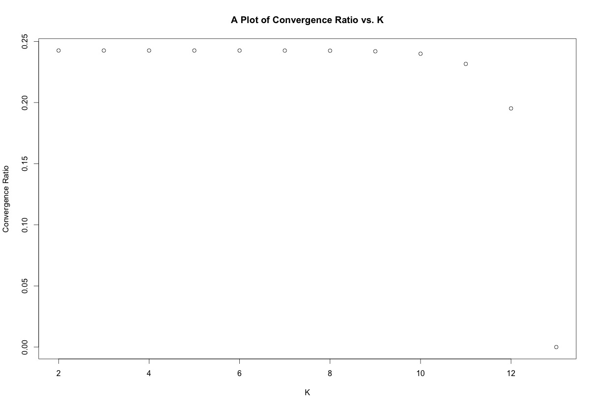
You can see the numerical solution matches the analytical solution found by the standard partial derivative method. The R function also outputs a plot of f(x) as a function of the iteration number as well as a plot of the convergence ratio, given by:
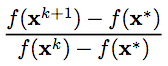 The plots for this function are shown below:

For fun I also created a simple function that uses the necessary and sufficient conditions to check if an x* derived from analytical procedures is a global minimum. The first condition to be a global minimum is that the gradient must be equal to zero. The second fact is that the Hessian matrix of a convex function must be positive semidefinite for all x.
However, if the Hessian can only be verified to be positive semidefinite for a ball of diameter 2*epsilon centered around a given x*, we can only be certain that x* is a local minimum.
On the other hand if the Hessian is not positive semidefinite we aren’t sure of much since we don’t know anything about the shape of the function. Finally, if the gradient is not zero we know for certain that we are not at a minimum since there is some direction we can travel that will lead to a lower f(x).
analyticTest <- function(func, x.star, convex = FALSE) {
  require(numDeriv)

  result <- try(hess <- hessian(func,x.star))
  if(class(result) == "try-error") {
    stop("Error: Make sure dimensions of function and x.star match.")
  }

  result <- try(grad <- round(grad(func,x.star),5))
  if(class(result) == "try-error") {
    stop("Error: Make sure dimensions of function and x.star match.")
  }

  if(!isTRUE(all(eigen(hess)[[1]]>0))) {
    print("Hessian matrix not semi-definite. x* not a local or global minimum.")
    print(1)
    return(FALSE)
    }

  else if(!isTRUE(all(grad == 0))) {
    print("Gradient at x star is not zero. x* not a local or global minimum.")
    print(2)
    return(FALSE)
    }

  else if(convex == TRUE) {
    print("x* is a global minimum.")
    print(3)
    return(TRUE)
    }

  else {
    print("x* may be a local or global minimum. Check convexity of function.")
    print(4)
    return(FALSE)
  }
}
