Postscript
I wrote this paper as part of an intentional finance class I took from UW’s school of public affairs. It’s not the best thing I’ve ever written, but there’s some decent analysis in it. I wrote it before I learned Adobe Illustrator so there are some pretty ridiculous looking graphics. As I remember, we were suppose to put ourselves in the place of a policy advisor. The heading for mine was “Report for Mr. Yiannis Stournaras, Greek Minister of Finance.”
Executive Summary and Problem Statement
On Thursday, 2 August 2012 Mario Draghi, head of the European Central Bank (ECB), held his latest press conference. “The euro is irreversible,” he said, “It stays…It is pointless to bet against the euro.”[1] However, Mr. Draghi also made it clear that the continued flow of funds to troubled countries would come with requirements for economic reform.[2] While he did not announce immediate ECB action, Draghi did state that in upcoming weeks the ECB would begin the purchase of short-term Greek bonds in a continued effort to help the Greek economy.
However, the austerity measures that have been required by the ECB, and by its informal umbrella institution, the Troika, have been unpopular with the Greek people. In addition to austerity, two economic alternatives have been suggested in recent months – internal devaluation and an exit from the Eurozone – each claiming to provide the best chance of resolving the now five-year long Greek recession. Is continued Troika assistance really the best alternative?
This report will outline four possible policy options for the Greek government moving forward. Included is one package of reforms that are recommended independent of the other three policy options:
- Maintaining the status quo and accepting Troika assistance
- Leaving the Eurozone and returning to the Greek drachma
- Defaulting on the current debt obligations
None of these solutions is perfect and all of them will require sacrifice and, likely, economic hardship in the short term. They also have varying degrees of political and social feasibility. After a detailed analysis it seems clear that the least harmful path is indeed Troika assistance including some form of austerity reforms. However, as will be suggested in the concluding recommendation, these reforms could possibly be restructured by negotiating with Troika officials. As unpopular as austerity has been with the Greek populace, other policy options would likely turn out to be equally unpopular and have the additional effect of hurting political relations between Greece and the rest of Europe.
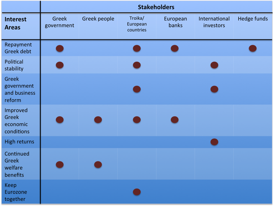
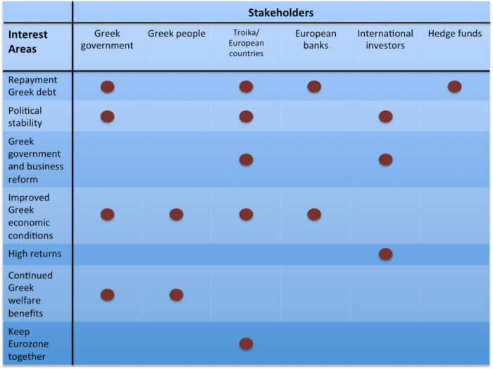
The stakeholder positions of the various groups involved in the Greek debt crisis are shown in the stakeholder map below. Note two things. First, the interests of the stakeholders are far from aligned. Second, these are the interests as they stand today. Hedge funds, for instance, having already locked in their investment portfolio with Greek debt, care about full repayment and little else. Meanwhile, the interest of the Troika and various European countries are more complex.
This is not to say that these are the interest as they should be. For instance, Greece should probably shift some portion of its interest away from maintaining Greek entitlement payments and toward more governmental and business reforms. The discussion in this report will make this point clear.
History

The current crisis in Greece is a confluence of factors including steadily increasing public debt, stagnant government revenue, large public sector obligations, a history of government corruption and low transparency, a poor business environment, all combined with a European-wide slowdown in output.
Greece enjoyed fairly strong growth from 2001 through 2007, but has been very hard hit in the years since the Euro crisis started. Problems worsened throughout 2009 and 2010 with the release of a series of budget deficit revisions, most notably a change in the 2009 figure, which began at 3.7% of GDP[3] and eventually topped out at 15.4%.[4]
This only increased suspicions of Greek corruption in a country that already ranked among the lowest countries in all of continental Europe in the Corruption Perceptions Index. Indeed, Greece’s ranking steadily decreased between 2009 and 2011.[5]
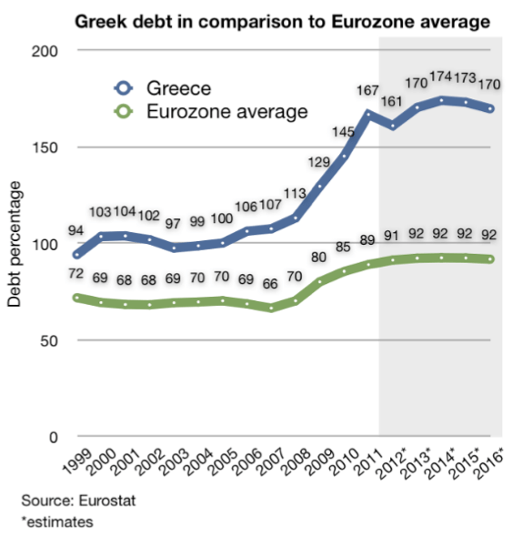
Unfortunately, Greece could ill afford such budget deficits, which added to an already mounting public debt that peaked at 167% of GDP in 2010. Government revenue, meanwhile, remained stagnate, hovering around 40% of GDP since 2001.[6]
Rather than decline, however, government expenditures have increased since 2008 from 45% to 50% of GDP.[7] This is a result of a shrinkage in GDP from the Greek recession, combined with a failure to adequately cut expenditures accordingly. A significant portion of government expenditure has been dedicated toward public employment and support programs. For instance, one report found that before the required ECB reforms, “On average, Greeks retired at 58 years old and received 96% of pre-retirement income.”[8]
As the Greek crisis worsened three financial institutions came together in what has become known as the Troika. These are the European Council, the ECB, and the International Monetary Fund (IMF). The Troika release two separate bailout funds: €110 billion in May of 2010 and a second €130 billion package in February of 2012.[9] All told, Greece debt stands at €356 billion.[10]
This brief history demonstrates the enormity of the problem facing Greece today. The following sections will discuss four separate policy options with the first being a set of necessary general reforms.
General Reforms
The current Troika loans are contingent on political and economic reforms that can be separated into two types. One type is a contentious set of so-called “internal devaluation” reforms. The other set contains a sensible set of government and business reforms that are long overdue. These should be undertaken regardless of the broader economic measures that will be discussed in the next part of this report. The Greek economy cannot plunge into a five-year recession and experience two elections in 2012 alone, only to keep things as they have been.
Tax reform
Tax payment is notoriously lax in Greece. Only about 25% of the €40 billion owed in taxes are collected annually.[11] The government can ill afford the loss of so much potential revenue in the middle of the worst debt crisis the country has ever seen. One option is to moderately reduce taxes, but drastically increase collection from 25% closer to the averages seen in most developed economies, thereby increasing government revenues while simultaneously giving concessions to tax payers.
Improved transparency
Greek political transparency must improve for its economic situation to improve. Greek government corruption has cost the country dearly, especially the fiscal budget deficits that were repeatedly covered up, leading to artificially high investment in Greece and worsening the credit situation. Implementation of consistent long-term measures to improve transparency and fiscal reporting will help restart foreign direct investment in Greece, but at levels that are commensurate with its true financial condition.
Business reform
Greece ranked 100 on the 2012 World Bank Doing Business Index. This is an extremely low ranking for a country of Greece’s stature and represents the significant challenges to starting and efficiently running a business in the country. The good news is that many other countries have made quick and substantial progress in reforming their own business environment. Such reform is necessary if Greece is to spur domestic and international investment, and would likewise improve the fortunes of the Greek people – 99.9% of businesses in Greece are small and medium-sized enterprises (SMEs).[12]
The government must also continue the fight against widespread abuse by business cartels. These cartels have caused prices in Greece to continue to rise even as the economy has shrunk by 13%.[13] This hurts consumers and limits the flexibility of government policy.
Benefits cuts
Public wages rose 50% between 1999 and 2007[14], an extraordinary rate. Cutting wages is a different discussion, but stopping the disproportionate increase in public sector wages is a necessary step to help stem the chronic deficit problem.
Keeping with the Status Quo
The first option is to maintain the current plan of receiving Troika bailouts and move forward with economic reforms. Again, one set of Troika requirements discussed above is necessary regardless of whether the rest of the bailout package reforms are accepted.
The second set of bailout reforms, geared toward creating a so-called “internal devaluation,” are more politically and socially contentious. The difficulty of these reforms has already come to light. After the June passage of an austerity package expected to save €28 billion, two days of violent riots ensued during which 300 protesters and police were injured.[15] Yet as of 4 August 2012 only 100 of the required 300 reforms had been completed.[16] Some of these are not set to take effect until 2013 or ‘14 and further Troika funding is unavailable until all 300 reforms are in place. Given the already widespread public discontent of the limited reform measures that have been enacted, when the full set are completely implemented public discontent is likely to grow, possibly resulting in further violence.
An internal devaluation uses internal structural changes to a country’s economic system in an effort to reduce production costs, and through this channel prices for goods. This improves competitiveness in world markets and increases exports, thereby spurring economic growth. As growth increases and public debts are reduced, the structural changes can be slowly reversed.
There are two possible methods to impose an internal devaluation. The first is a mandated decrease in wages, while the second uses adjustments to payroll and value added taxes (VAT).
In first the method, wages are reduced, inducing a recession, but lowering production costs and increasing exports, eventually reversing the recession and restarting economic growth. This strategy is not unprecedented as a solution to the worldwide financial crisis. Estonia embarked on such a path throughout the past few years. In Estonia, internal devaluation led to 2010 GDP growth of 2.3%; by 2011 growth stood at an impressive 7.5%![17] Additionally, public debt in Estonia is now far below any other Euro country. However, it is important to remember that the political and social situation in Estonia is far different than that in Greece.
Growth did come in Estonia, but it was preceded by several years of economic hardship as its leaders refused to borrow and instead fought to keep government spending low. Initially, GDP dropped by over 14% in 2009 and unemployment hit 16%.[18] Estimated GDP loss for Greece is 15.8% if the current internal devaluation measures continue, but could be much worse.[19] Unemployment in Greece is already 22% and could easily slip even higher if events in Estonia are a precedent. Nevertheless, it is this first method that the Troika has so far favored.
The second method of devaluation is to encourage exports more “stealthily” by increasing the VAT and decreasing payroll taxes.[20] This second method keeps wages at their current levels while also keeping operating revenue roughly the same (since income taxes are unchanged). At the same time the lower payroll tax decreases production costs significantly – in Greece the employer contributes 28% of wages toward such taxes.[21] Additionally, a higher VAT discourages consumption of imports leading to a positive balance of trade. The hope is that in the long run payroll taxes can rebound or other forms of public support can be found to recoup the necessary short-term loss to the social security fund, eventually refilling the fund before permanent cuts to entitlements are required. This second method seems to be more politically and social feasible, but would require a renegotiation of the bailout reforms as they currently stand.
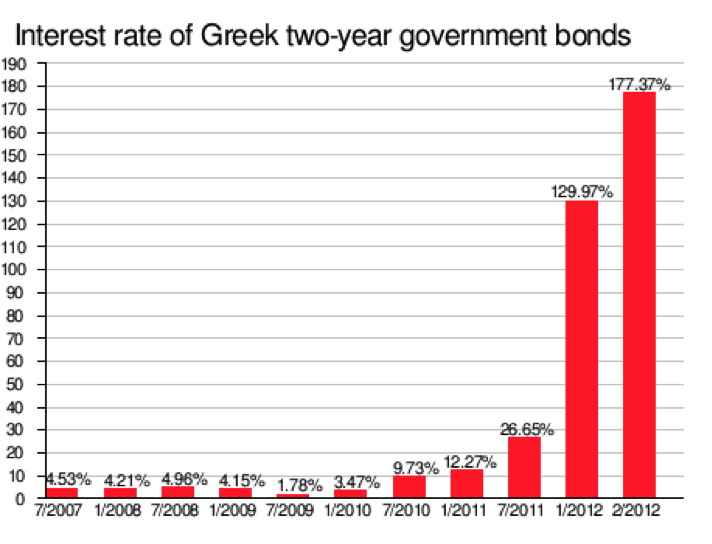
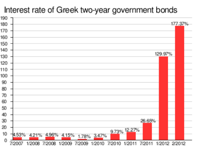
Troika action has by no means been all bad, however. Greek banks have been heavily reliant on the ECB for liquidity during the crisis and even during the pre-crisis era 2.5% of Greek GDP came from EU transfer payments.[22] Additionally, the recent ECB announcement of the purchase of short-term Greek debt seems reasonable given the extraordinary increase in Greek two-year bond yields. Combined with the €240 billion in bailout funds and consistently strong rhetoric of Euro survival, it seems clear that overall the Troika is committed to seeing Greece, and indeed the Eurozone, succeed. Likewise, austerity is not an unreasonable reform considering the state of Greek public debt, revenue, and expenditure. Austerity of some kind will be required, although the degree and form it takes may be able be negotiated with the Troika.
Leaving the Eurozone
Leaving the Eurozone would involve a return to the drachma and subsequent currency devaluation. Greek exports would increase and this would improve economic prospects in the medium and long run. Again, in the short term a recession is likely since domestic wealth and savings are decreased by the devaluation at the same time that imports would become more expensive. As a result, aggregate demand would likely fall in the immediate aftermath of the devaluation. This is somewhat offset, however, by an increase in exports and tourism in the short run, and in the long run it is suggested that these two factors would together pull the country out of the recession and restore long-term economic growth.
Additionally, a move to the drachma would mean an increase in the debt overhang – the amount of debt that Greece owes to foreign creditors. This increase is due to the fact that most Greek debt is denominated in foreign currencies and so cannot be devalued along with the domestic currency. Additionally, this foreign denomination means the debt cannot be “inflated away” with loose monetary policy after a return to the drachma as is true when debt is domestically held or otherwise denominated in the domestic currency.
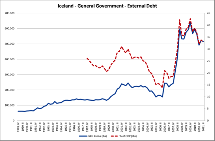
An analogy to Iceland is instructive as to the possible consequences of increased debt overhang. In 2008 Iceland began a devaluation of its currency, the Krona. As the chart below demonstrates, the external debt shot up to roughly three times its previous levels.

Greece would have to either negotiate a payment of its debts in drachma – at an unfavorable drachma to Euro exchange rate – or purchase Euro itself on the open market in order to repay its obligations. Obviously, this would be a great burden on the Greek economy. One option that could be used in conjunction with an exit from the Eurozone is a debt default, which will be discussed in the next section. If Greece chooses not to default, it would have to service its debt at regular intervals, which would entail a substantial regular payment from Greece to its creditors.
This increase in debt must be weighed against the simultaneous increase in Greek tourism and exports. After its devaluation, for instance, Iceland was considered a “bargain” as a travel destination.[23] A full quarter of Greek GDP comes from tourism[24] and a significant increase in tourism could indeed be great news for growth. This is especially true if a return to the drachma is viewed by the Greek people as a superior policy, and therefore leads to more social and political stability and an end to rioting and protests, which otherwise would most certainly discourage tourism.
On the whole, however, the merits of a devaluation may be less significant than has been suggested in other reports. Imports account for 30% of Greek GDP and are mostly inelastic – goods that customers are reluctant to cut back on even if they increase in price – such as oil, food, and pharmaceuticals.[25] Exports, meanwhile, only account for 25% of GDP; and some major export industries, such as shipping, are dollar denominated and therefore immune from a drachma devaluation and its otherwise lowering of prices.[26] Together, this may mean that the relatively more expensive imports caused by a devaluation outweigh the benefits of cheaper exports, perhaps making the economic situation worse, not better.
Lastly, the logistics of a Eurozone exit are challenging, but certainly not impossible. First, Greece would have to take a so-called “banking holiday,” temporarily freezing the banking sector to stop capital from leaving the country in anticipation of a drachma reinstatement. Next, over a period of several days the government would set an exchange rate and redenominate the banking sector into drachma. After banks reopened, Greek citizens could go to any branch and exchange their Euro for drachma, which the government would have to print and distribute to banks. Producers would also have to update all of their prices in terms of drachma.
Loan Default
A third option is a loan default. Under this plan, Greece would decide not to pay back any of its debts, or, alternatively, pay back carefully selected loans – perhaps those held domestically, for instance – thereby reducing public debt substantially. This plan is not an option if continued Troika funding is desired and in practice it would likely be combined with a Eurozone exit and drachma devaluation.
A more ideal option would be to structure a large-scale debt write down, but such a debt restructuring already took place in March of 2012 when private bond holders of Greek debt voluntarily agreed to take a 53% loss totaling €105 billion.[27] It is unlikely, then, that there is remaining low-hanging fruit, as it were, when it comes to renegotiating debt. Pay back or complete default seem to be the only two possible scenarios at the moment.
The obvious benefit of this approach is the drastic reduction of the large Greek debt. Combined with a currency devaluation, it would avoid the debt overhang problem and provide an opportunity for economic recovery. Such a strategy would drastically increase the cost of borrowing, however, and would shut Greece out of international lending markets for several years at a minimum.
The reason a Eurozone exit is inevitable under a default is simple. Suppose for a moment that Greece did not exit the Euro. Since revenues are not yet covering government expenditures, and because borrowing would no longer be an option, a default would mandate immediate measures to balance the budget. This would entail either raising taxes, laying off public sector workers, cutting welfare benefits, or some combination of the three.[28] Greek banks would also loose Eurozone loan support, resulting in a failure to recapitalize and insolvency, quickly leading to a large number of bank failures.[29] Together these factors would induce a deep recession and would likely result in widespread riots and violence.[30] However, combined with a return to the drachma and devaluation, these events could be avoided or dampened.[31] However, this plan is still subject to the economic weaknesses of a return to the drachma that were outlined in the previous section.
There are other concerns in defaulting as well. A default would likely hurt political relationships with other European countries. A substantial amount of Greek debt is held either by other European governments or by private banks in European countries. Together US$44.3 billion is held in France, US$13.3 billion in Germany, US$10.5 billion in the UK, and combined Italy, Switzerland, and Span hold approximately US$5 billion.[32] Defaulting on those creditors would undoubtedly cause negative shocks throughout their national economies, and the move would be seen as fiscally irresponsible, perhaps even leading to a breakdown of normalized political relations with other members of the EU.
Lastly, a default might also mean the seizure of Greek assets abroad as foreign governments, private banks, and, especially, hedge funds – which also hold several billion in Greek debt – attempt to recoup their losses.[33] Some hedge funds, known colloquially as “vulture funds,” make seizing assets an explicit strategy.[34] And seizures are quite common throughout history having occurred in other sovereign defaults involving Brazil, Peru, Liberia, Zambia, and the Democratic Republic of the Congo, to name just a few.[35]
Recommendation
Ultimately, remaining with the status quo appears to be the most politically feasible policy available and offers the best chance at economic success. The New Democracy Party, which was elected 17 June 2012, ran on a pro-bailout platform and garnered the highest percentage of votes from the Greek electorate.[36] Investors worldwide reacted positively to this news[37] and it is important to continue to demonstrate political follow-through and stability going forward by keeping with the policy platform on which the party was elected.
Thus far, riots, sometimes violent, have not been uncommon. But the Troika is likely sensitive to the political stability of Greece and does not desire nationwide Greek violence any more than the incumbent Greek government. If discontent among Greeks grows to the point that the radical Syriza party – which has a contentious relationship with the rest of Europe[38] – is likely to win election, or, worse, a coup is forecast, the Troika would likely be willing to postpone or reduce austerity measures. In the end, of course, some austerity is necessary for the Greek economy to recover. Likewise patronage, business cartels, and government corruption must be rolled back. All of these measures will temporarily hurt some segment of the Greek populace, but in exchange long-term economic health is likely to be stronger. It is up to Greek politicians to sell this idea to the people.
The Troika and individual European nations, most notably, Germany, do not always agree on the best European-wide economic policy. However, in the final analysis they are both committed to Greek success. A Greek default or Eurozone exit would ripple throughout Europe, causing investor panic in Spain, Italy, and Portugal, eventually spreading to France and Germany.[39] For this reason, Greece has some leverage over the Troika and can perhaps use this power to negotiate a reduced set of austerity requirements. Specifically, an internal devaluation using the VAT and payroll tax method is politically and socially preferable to the Troika’s current wage reduction plan. One further suggestion, then, is to take this change to the Troika using Greek social resistance and possible riots as leverage.
Whatever happens, Greece has a tough line to walk between the desires of the Greek people and the reforms proposed by the Troika. This line, though, is still preferable to Greece turning its back on the rest of Europe as would be necessary in a return to the drachma or currency devaluation. In this particular case, what is best for the Eurozone is what is also best for the Greek government and people.
Charts and Graphs
All charts and graphs besides the Stakeholder map, which I created, are sourced from Wikipedia.
Endnotes
[1] Jones, Johnson, and Watkins, “Draghi Kills Hope of Instant Action.”
[2] “Draghi’s Bold Move in Euro Chess Game.”
[3] Catao, Fostel, and Ranciere, “Fiscal Discoveries, Stops and Defaults.”
[4] Jolly, “2009 Greek Deficit Revised Higher.”
[5] “Transparency International – Country Profiles.”
[6] Eurostat, “Government Revenue, Expenditure and Main Aggregates.”
[7] Ibid.
[8] Roscini, Schlefer, and Dimitriou, “The Greek Crisis: Tragedy or Opportunity?”.
[9] The Associated Press, “Key Dates in Greece’s Debt Crisis.”
[10] “Q&A.”
[11] “The Greek Economy.”
[12] Hyz, “Small and Medium Enterprises (SMEs) in Greece – Barriers in Access to Banking Services. An Empirical Investigation.”
[13] “The Greek Economy.”
[14] “Q&A.”
[15] The Associated Press, “Key Dates in Greece’s Debt Crisis.”
[16] “The Greek Economy.”
[17] Greeley, “Krugmenistan Vs. Estonia.”
[18] Ibid.
[19] Weisbrot and Montecino, “More Pain, No Gain for Greece.”
[20] Editors, “Greece’s Least Bad Option Looks to Be Internal Devaluation.”
[21] Wikipedia contributors, “Taxation in Greece.”
[22] “Greece.”
[23] “With Devaluation of the Krona, Iceland Is Now a Hot Spot.”
[24] “Greece.”
[25] Ibid.
[26] Ibid.
[27] Wikipedia contributors, “Greek Government-debt Crisis.”
[28] Giles, Birkett, and Jones, “Consequences of a Greek Eurozone Exit.”
[29] Ibid.
[30] Ibid.
[31] Ibid.
[32] “Q&A.”
[33] “Greece.”
[34] Ibid.
[35] Ibid.
[36] Brown, “Greek Elections.”
[37] Ibid.
[38] Ibid.
[39] Giles, Birkett, and Jones, “Consequences of a Greek Eurozone Exit.”
Bibliography
Brown, Abram. “Greek Elections: Investors, Take A Moment To Cheer Pro-Bailout Party’s Victory – Forbes.” Forbes, June 17, 2012. http://www.forbes.com/sites/abrambrown/2012/06/17/greek-elections-investors-take-a-moment-to-cheer-pro-bailout-partys-victory/.
Catao, L., A. Fostel, and R. Ranciere. “Fiscal Discoveries, Stops and Defaults.” (2011). http://www.parisschoolofeconomics.eu/IMG/pdf/Catao-Fostel-Ranciere-oct2011.pdf.
“Draghi’s Bold Move in Euro Chess Game.” Financial Times, August 2, 2012. http://www.ft.com/intl/cms/s/39ff72c0-dcab-11e1-a304-00144feab49a,Authorised=false.html?_i_location=http%3A%2F%2Fwww.ft.com%2Fcms%2Fs%2F0%2F39ff72c0-dcab-11e1-a304-00144feab49a.html&_i_referer=#axzz22LATAiaq.
Editors, the. “Greece’s Least Bad Option Looks to Be Internal Devaluation: View.” Bloomberg, n.d. http://www.bloomberg.com/news/2012-01-04/greece-s-least-bad-recovery-option-looks-to-be-internal-devaluation-view.html.
Eurostat. “Government Revenue, Expenditure and Main Aggregates”, n.d. http://appsso.eurostat.ec.europa.eu/nui/show.do?query=BOOKMARK_DS-054156_QID_-76724309_UID_-3F171EB0&layout=TIME,C,X,0;GEO,L,Y,0;UNIT,L,Z,0;SECTOR,L,Z,1;INDIC_NA,L,Z,2;INDICATORS,C,Z,3;&zSelection=DS-054156UNIT,PC_GDP;DS-054156INDICATORS,OBS_FLAG;DS-054156INDIC_NA,B9;DS-054156SECTOR,S13;&rankName1=SECTOR_1_2_-1_2&rankName2=INDIC-NA_1_2_-1_2&rankName3=INDICATORS_1_2_-1_2&rankName4=UNIT_1_2_-1_2&rankName5=TIME_1_0_0_0&rankName6=GEO_1_2_0_1&pprRK=FIRST&pprSO=PROTOCOL&ppcRK=FIRST&ppcSO=ASC&sortC=ASC_-1_FIRST&rStp=&cStp=&rDCh=&cDCh=&rDM=true&cDM=true&footnes=false&empty=false&wai=false&time_mode=ROLLING&lang=EN&cfo=%23%23%23%2C%23%23%23.%23%23%23.
Giles, Chris, Russell Birkett, and Cleve Jones. “Consequences of a Greek Eurozone Exit.” Financial Times, May 21, 2012. http://www.ft.com/intl/cms/s/2/0a35504a-0615-11e1-a079-00144feabdc0.html#axzz22zmX3gKi.
“Greece: Better To Stay Put In Euro?” Seeking Alpha, n.d. http://seekingalpha.com/article/646871-greece-better-to-stay-put-in-euro.
“Greece: Here Come the Vulture Funds.” The Guardian, May 17, 2012. http://www.guardian.co.uk/commentisfree/2012/may/17/greece-vulture-funds.
Greeley, Brendan. “Krugmenistan Vs. Estonia.” BusinessWeek: Global_economics, July 20, 2012. http://www.businessweek.com/articles/2012-07-19/krugmenistan-vs-dot-estonia#p1.
Hyz, Alina. “Small and Medium Enterprises (SMEs) in Greece – Barriers in Access to Banking Services. An Empirical Investigation.” International Journal of Business and Social Science 2, no. 2 (February 2011).
Jolly, David. “2009 Greek Deficit Revised Higher.” The New York Times, November 15, 2010, sec. Business Day / Global Business. http://www.nytimes.com/2010/11/16/business/global/16deficit.html.
Jones, Claire, Miles Johnson, and Mary Watkins. “Draghi Kills Hope of Instant Action.” Financial Times, August 2, 2012. http://www.ft.com/cms/s/c07cf4d2-dc86-11e1-bbdc-00144feab49a,Authorised=false.html?_i_location=http%3A%2F%2Fwww.ft.com%2Fcms%2Fs%2F0%2Fc07cf4d2-dc86-11e1-bbdc-00144feab49a.html&_i_referer=#axzz22bccWj8w.
“Q&A: Greek Debt Crisis.” BBC, June 18, 2012, sec. Business. http://www.bbc.co.uk/news/business-13798000.
Roscini, Dante, Jonathan Schlefer, and Konstantinos Dimitriou. “The Greek Crisis: Tragedy or Opportunity?” Harvard Business School, September 16, 2011.
The Associated Press. “Key Dates in Greece’s Debt Crisis.” BusinessWeek: Undefined, June 15, 2012. http://www.businessweek.com/ap/2012-06-15/key-dates-in-greeces-debt-crisis.
“The Greek Economy: Promises, Promises.” The Economist, August 4, 2012. http://www.economist.com/node/21559974?zid=307&ah=5e80419d1bc9821ebe173f4f0f060a07.
“Transparency International – Country Profiles”, n.d. http://www.transparency.org/country.
Weisbrot, M., and J. A. Montecino. “More Pain, No Gain for Greece: Is the Euro Worth the Costs of Pro-Cyclical Fiscal” (2012). http://gesd.free.fr/paingain.pdf.
Wikipedia contributors. “Greek Government-debt Crisis.” Wikipedia, the Free Encyclopedia. Wikimedia Foundation, Inc., August 10, 2012. http://en.wikipedia.org/w/index.php?title=Greek_government-debt_crisis&oldid=506652815.
———. “Taxation in Greece.” Wikipedia, the Free Encyclopedia. Wikimedia Foundation, Inc., August 3, 2012. http://en.wikipedia.org/w/index.php?title=Taxation_in_Greece&oldid=494104235.
“With Devaluation of the Krona, Iceland Is Now a Hot Spot.” U-T San Diego, n.d. http://www.utsandiego.com/news/2009/jan/04/1t04advicem18931-no-headline/.


 -norm while lasso regression uses the
  -norm. Specifically the forms are shown below.
 The only difference is the
  term. I read (or heard) somewhere that ridge regression was originally designed to deal with invertability issues in OLS. By adding the small
  is close to zero the ridge solution approachese the least squares solution. As
 axis (in this case). The contours inscribed by the solutions (the red circles) can easily intersect the diamond at it’s tip and force
  to zero. This is much more unlikely in the case on the right for ridge regression where the
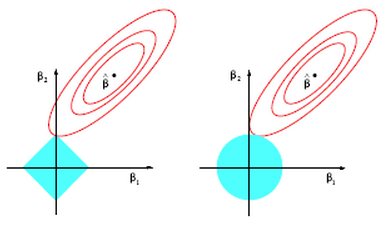


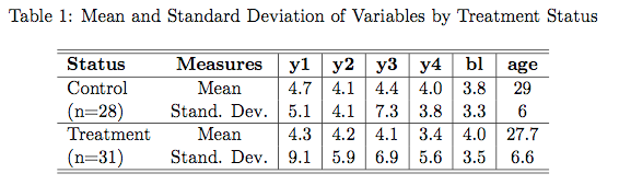


 (
( ) possible models (including the null model with only the intercept). To give a sense of how large that is, it’s beginning to approach the number of starts in the observable universe (
 ). Even modern computers would take too long to test every possible model.