Percolation Algorithm In R

I’m casually following along with a few of the lessons in Princeton’s Algorithms, Part 1 on Coursera. The course itself is taught in Java, but I thought completing some of the lessons in R would improve my R skills. The first activity I’ve completed is a percolation simulation using weighted quick-union with path compression. I’m not actually sure if this was one of the assignments, but it seemed cool so I thought I’d give it a try.

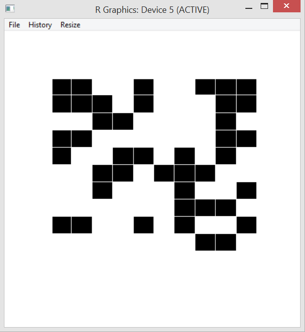
Percolation is meant to model physical or social systems where some type of blockage occurs. The algorithm taught in the class is to begin with full blockage and to randomly unblock one element until there is a path from one side of the system to another. The simplest method of doing this is to imagine a blocked grid. The initial blocked system is shown below.

percolation start

My algorithm removes one blockage per half second and this is modeled by turning the black box white. A totally percolated system is shown below. Notice there is now a path through the blockage – by starting at the bottom, following the open (white) squares up and to the left and then diagonally up and to the right.

percolation end

At the moment percolation is completed a message is printed to the console.

percolation output

The code to initialize the board and percolated system and to run the clearing algorithm is shown below.

####################################################################
# James McCammon
# 21 Feb 2015
# Percolation Algorithm Functions Version 1
####################################################################
# Load libraries
library(shape)
source("perc_functions.R")
 
# Define variables
nrows = 10
ncols = 10
nsites = nrows*ncols
closedSites = 1:nsites
numneighbors = 4
display = NULL
#display = matrix(data=0, nrow=nrows, ncol=ncols)
VTN = nsites + 1
VBN = nsites + 2
 
# Initailize board
board = initBoard()
initDisplay()
initVTN()
initVBN()
 
# Run main
main()

Created by Pretty R at inside-R.org

Most of the work is done in the set of functions below. This can definitely be improved, for example by incorporating an arbitrary list of neighbors into each site object rather than assuming the system is a square grid and determining neighbors by looking in the four quadrants around each site. I could also think harder about memory usage. Right now I just threw everything into the global environment and didn’t think too hard about memory usage or efficiency. Using the tracemem() function from the pryr shows there are a few times the board object is copied. I’ll probably play around with things and continue to improve them.

####################################################################
# James McCammon
# 21 Feb 2015
# Percolation Algorithm Main Version 1
####################################################################
# Define main function
main = function() {
  sleeptime = 0.5
 
  while(!connected(VTN, VBN)) {
    randSite = getRandSite()
    board[[randSite]]$open = TRUE
    #location = trans2display(randSite)
    #write2display(location)
    filledrectangle(mid=c(display[[randSite]]$xmid, 
                          display[[randSite]]$ymid), 
                    display[[randSite]]$wx, 
                    display[[randSite]]$wy, 
                    col='white', 
                    lwd=1, 
                    lcol='white')
 
    neighbors = getNeighbors(randSite)
 
    for(i in 1:numneighbors) {
      if(is.null(neighbors[[i]])) next
      if(!isOpen(neighbors[[i]])) next
      join(randSite, neighbors[[i]])
    } 
    Sys.sleep(sleeptime)
  }
  print("Percolation completed")
  p = 1 - (length(closedSites)/nsites)  
  return()
}
 
 
#Initalize the display
initDisplay = function() {
  display <<- as.vector(1:nsites, mode='list')
  windows(5, 5)
  plot.new()
  xmid = 0
  ymid = 1
  wx = .1
  wy = .1
  index = 1
 
  for(row in 1:nrows) {
    for(col in 1:ncols) {
      filledrectangle(mid=c(xmid, ymid), wx=wx, wy=wy, col='black', lwd=1, lcol='white')
      display[[index]] <<- list('xmid'=xmid, 'ymid'=ymid, 'wx'=wx, 'wy'=wy)
      index = index + 1
      xmid = xmid + .1
    }
    xmid = 0
    ymid = ymid - .1
  }  
}
 
 
# Gets root 
getRoot = function(node) {
  while(node != board[[node]]$root) {
    board[[node]]$root <<- board[[board[[node]]$root]]$root
    node = board[[node]]$root
  }
  return(node)
}
 
 
# Checks if two notes are connected
connected = function(node1, node2) {
  return(getRoot(node1) == getRoot(node2))
}
 
 
# Initalize board
initBoard = function() {
  board = as.vector(1:nsites, mode='list')
  board = lapply(board, function(i) list("index"=i, "size"=1, "root"=i, "open"=FALSE))
  return(board)
}
 
 
# Initalize virtural top node
initVTN = function() {
  board[[VTN]] <<- list("index"=VTN, "size"=(ncols + 1), "root"=VTN, "open"=FALSE)
  lastrow = nsites - ncols + 1
  for(i in 1:ncols)  {
    board[[i]]$root <<- board[[VTN]]$root
  }  
}
 
 
# Initalize virtual bottom node
initVBN = function() {
  board[[VBN]] <<- list("index"=VBN, "size"=(ncols + 1), "root"=VBN, "open"=FALSE)
  lastrow = nsites - ncols + 1
  for(i in lastrow:nsites) {
    board[[i]]$root <<- board[[VBN]]$root
  }  
}
 
 
# Choose random site
getRandSite = function() {
  randSite = sample(closedSites, size=1)
  closedSites <<- closedSites[-which(closedSites==randSite)]
  return(randSite)
}
 
 
# Checks if site is open
isOpen = function(site) {
  return(!(site%in%closedSites))
}
 
 
# Get neighbors on a square board
getNeighbors = function(index) {
  top = index - ncols
  if(top < 1) top = NULL
 
  bottom = index + ncols
  if(bottom > nsites) bottom = NULL
 
  left = index - 1
  if(!(left%%ncols)) left = NULL
 
  right = index + 1
  if(right%%ncols == 1) right = NULL
 
  return(list("tn"=top, "rn"=right, "bn"=bottom, "ln"=left))
}
 
 
# Join two nodes
join = function(node1, node2) {
 
  r1 = getRoot(node1)
  r2 = getRoot(node2)
  s1 = board[[r1]]$size
  s2 = board[[r2]]$size
 
  if(s1 > s2) {
    board[[r2]]$root <<- board[[r1]]$root
    board[[r1]]$size <<- s1 + s2
  }
 
  else {
    board[[r1]]$root <<- board[[r2]]$root
    board[[r2]]$size <<- s2 + s1 
  } 
}
 
 
####################################################################
# Functions for visualizing output with matrix
####################################################################
# Translate location of site to matrix
trans2display = function(index) {
  col = index%%ncols
  if(!col) col=ncols
  row = ceiling(index/nrows)
  return(list("row"=row, "col"=col))  
}
 
 
# Update the matrix display
write2display = function(transObject) {
  display[transObject$row, transObject$col] <<- 1  
}

Created by Pretty R at inside-R.org

Shiny Web App

I’ve created my first Shiny web app! The web app takes in a .csv or Excel file of short URLs and returns the full URLs. This can be a necessary process in some web analysis and can take many hour to do by hand if there are thousands of links (as there often are). A screenshot of the web app is below. And you can use the web app by going here:

https://jamesmccammon.shinyapps.io/Forward_Links

Shiny App FwdLinks Screenshot

The web app allows input in .csv and Excel formats and also allows the user to export the full URLs in .csv and Excel formats. If an Excel file is used as input a drop down menu automatically appears so the user can select the appropriate worksheet. There is also a progress bar and error handling in case something goes wrong.

A Shiny web app is composed of two files: a user interface file – ui.R – and a server file – server.R. Shiny was recently updated to allow a single file to contain both functions, but I prefer keeping the files separate for clarity. There is a separate function (not shown here) I wrote in R to get the forward URLs.

ui.R is below.

require(shiny)
 
shinyUI(fluidPage(
  titlePanel("Get Full URLs"),
 
  tags$head(
    tags$style(HTML("   
      .errortext {
        font-size: 1em;
        color: red;
        padding-top: 1em;
        padding-bottom: 1em;
      }
    "))
  ),
 
  sidebarLayout(
    sidebarPanel(
      p('In web analytics it is somtimes necessary to transform short URLs into the full
        URL path. For instance, Twitter users often post URLs that are shortned with 
        Bitly, Ow.ly, Tr.im, or other URL shortening web apps. When doing analysis, however,
        you may want to determine the full URL.'), br(),
 
 
      h5('Step 1: Upload the file with short URLs'),
      radioButtons(inputId = 'inputformat',
                   label = 'What type of file are you uploading?',
                   choices = c('Excel' = 'excel', 'CSV' = 'csv')),         
      numericInput(inputId = 'datacol',
                   label = 'Which column are the short URLs in?',
                   value = 1,
                   min = 1,
                   max = 10,
                   step = 1), br(), br(),      
      helpText('Does the short URL column have a header row?'),
      checkboxInput(inputId = 'dataheader',label = 'Yes',value = TRUE), br(),
      fileInput(inputId = 'datafile', label = ''),
      uiOutput('worksheets'), 
 
      h5('Step 2: Get the full URLs'),
      actionButton(inputId = "getlinks", label = "Get Full URLs!", icon = icon("mail-forward")), br(), br(),
 
 
      h5('Step 3: Download the data'),
      radioButtons(inputId = 'outputformat',
                   label = 'In what format would you like to download the data?',
                   choices = c('Excel' = 'excel', 'CSV' = 'csv')),
      downloadButton('downloadlinks','Download Full URLs')      
      ),
 
    mainPanel(
      #textOutput('testing'),  
      h4('How to use this web app'),
        p(strong('Step 1:'), 'Upload a list of short URLs in .csv, .xls, or .xlsx format.
          The data should be in "long format" (sequential rows of a single column).
          If an Excel file is uploaded a dropdown menu will appear so that you can 
          select the appropriate worksheet.'),
        p('There are three tabs to view data. The first shows a summary of the 
          uploaded data file. The second shows the first 10 rows of the the shortened URLs. 
          The third will be blank until the forward URLs are processed.'),
        p(strong('Step 2:'), 'Click "Get Forward URLs" to get the full URLs from their shortened version. 
          This may take several minutes depending on the number of URLs to process. A progress 
          bar will appear along the top of the page that shows the percentage of URLs processed.'),
        p(strong('Step 3:'), 'After the foward urls are processed the file can be downloaded in .csv or .xlsx 
          format by clicking "Download."'),
        a('Click here to download test files', 
          href= 'https://www.dropbox.com/sh/tq2amcgfm7o99qi/AABrJVU4mNquOw-zmmRbRcaMa?dl=0',
          alt = 'Link to public Dropbox account with test files',
          target = '_blank'), br(), br(),
 
      uiOutput('errortext'),
 
      tabsetPanel(id = "datatabs",
                  tabPanel(title = "Data Summary", value = 'datasumtab', tableOutput('inputsum')),          
                  tabPanel(title = "Input Data", value = 'inputdatatab', tableOutput('inputdata')),
                  tabPanel(title = "Output Data", value = 'outputdatatab', tableOutput('outputdata'))
      )
    )  
  )
))

Created by Pretty R at inside-R.org

And here is server.R.

######################################################
# James McCammon
# 28 December 2014
# Get Full URLs function
# Version 4
######################################################
 
# Load libraries and source functions
require(shiny)
require(RCurl)
require(XML)
require(XLConnect)
source("functions.R")
 
# Define server instance
shinyServer(function(input, output, session) {
 
  # Initialize reactive values 
  values = reactiveValues()
 
  # Function to get file path of uploaded file
  filepath = reactive({
    file = input$datafile
    if(is.null(file)) return()
    return(file$datapath)
  })
 
  # If the uploaded file is Excel create a dropdown menu so the user can select the
  # worksheet with the relevant data.
  observe({
    if(is.null(input$dynamicinput)) {
      if(input$inputformat == 'excel' & !is.null(filepath())) {
        possibleerror = try(values$workbook <- loadWorkbook(filepath()), silent = TRUE)
        if(class(possibleerror) == 'try-error') { seterror('excelloaderror'); return() }
        sheetNames = getSheets(values$workbook)
        output$worksheets = renderUI({
          selectInput(inputId = "dynamicinput", 
                      label = "Select Worksheet",
                      choices = c(sheetNames,'Select' = 'select'),
                      selected = 'select')    
        })
      }
    }
  })
 
  # Create a table with summary data of the file
  output$inputsum = renderTable({
    if(is.null(input$datafile)) return()
    return(input$datafile)
  })
 
  # Create a table with the first 10 rows of the input data
  output$inputdata = renderTable({
    if(is.null(input$datafile) | is.na(input$datacol)) return()
      clearerror()
      # Load the relvant data depending on the file type. If the specified file type doesn't
      # match the loaded file throw an error.
      inputdata = switch(input$inputformat,
                   'excel' = {
                     if(is.null(input$dynamicinput)) return()
                     if(input$inputformat == 'excel' & input$dynamicinput == 'select') return()
                     tryCatch({ readWorksheet(values$workbook, sheet = input$dynamicinput, header = input$dataheader)
                     }, error = function(e) { seterror('excelreaderror'); return() })
                   },
                   'csv' = {
                     tryCatch({ read.csv(file = filepath(), header = input$dataheader, stringsAsFactors = FALSE)
                     }, error = function(e) { seterror('csvloaderror'); return() })
                   })
      # Take the data and get out the first 10 rows. If there is an error it's likely because
      # the specified worksheet or data column has no data. Tell the user this if an error occurs.
      values$inputdata = inputdata
      possibleerror = try(inputdata <- inputdata[[input$datacol]], silent = TRUE)
      if(class(possibleerror) == 'try-error') { seterror('subscripterror'); return() }
      inputdata = as.data.frame(inputdata[1:10])
      names(inputdata)[1] = "short_url_preview" 
      return(inputdata)   
  })
 
  # When the users pushes the "Get Full URLs" button get the URLs by calling the getFWLinks function
  # found in Functions.R. If there is no inpupt data let the user know they forgot to load it.
  observe({
    input$getlinks
    if(input$getlinks == 0) return()
    else {
      updateTabsetPanel(session, inputId = "datatabs", selected = "outputdatatab")
      output$outputdata = renderTable({
      possibleerror = try(values$output <- isolate(getFwLinks(as.data.frame(values$inputdata), input$datacol)), silent = TRUE)
      if(class(possibleerror) == 'try-error') { seterror('nodataerror'); return() }  
      return(as.data.frame(values$output[1:10,]))  
      })  
    }
  })
 
  # When the user selects "Download Full URLs" download them in the specified format.
  # Note the file.rename function is used to handle the temporary filepath created by Shiny.
  output$downloadlinks = downloadHandler(
    filename = function() {
      filename = switch(input$outputformat,
                        'excel' = 'Full_URLs.xlsx',
                        'csv' = 'Full_URLs.csv'
                        )
    },
    content = function(file) {
      if(input$outputformat == 'csv') {
        write.csv(values$output, 'temp.csv', row.names = FALSE)
        file.rename('temp.csv', file)    
      } 
      else {
        outputdata = loadWorkbook('temp.xlsx', create = TRUE)
        createSheet(object = outputdata, name = 'Full_URLs')
        writeWorksheet(outputdata, data = values$output, sheet = 'Full_URLs')
        saveWorkbook(outputdata, 'temp.xlsx')
        file.rename('temp.xlsx', file)    
      }
    }
  )
 
  # Create a function to ouput various error messages
  seterror = function(error) {
    errormessage = switch(error,
                    'excelloaderror' =  'Error: There was an error loading the file. 
                                         Are you sure it is an Excel file? Try changing
                                         your selection to CSV.',
                    'excelreaderror' =  'Error: The workbook loaded, but there was
                                         an error reading the specified worksheet',
                    'csvloaderror'   =  'Error: There was an error loading the file. 
                                         Are you sure it is a csv file?',
                    'fullurlserror'  =  'Error: There was a problem getting the full URLs.
                                         Are you sure you selected the correct data column?',
                    'subscripterror' =  'Error: There does not seem to be any data there.',
                    'nodataerror'    =  'Error: Did you forget to upload data?')
 
    output$errortext = renderUI({
      tags$div(class = "errortext", checked = NA, 
               tags$p(errormessage))
    })
  }
 
  # Define a function to clear error messages.
  clearerror = function() {
    output$errortext = renderUI({
      p('')
    })
  }  
})

Created by Pretty R at inside-R.org

Twitter Data!!!

I wanted to experiment with getting some Twitter data over the Thanksgiving break for one of my clients that does a fair amount of retail sales. I connected to the Twitter public stream using the “streamR” package and filtered based on around 30 hashtags. The idea was – well is, Cyber Monday is only just ending – to import the data into CartoDB. I tried this with some sample data from Twitter without worrying about filtering by hashtag and it looked great (CartoDB seems to be a pretty great tool). This “analysis” is more of what I like to call a “bonus treat” than actionable data, but why not have some fun. And who knows, maybe in analyzing the data some interesting trends will pop out. The final batch of data is just finishing up (I collected 8 .json files to make sure the file sizes were manageable since this is an experiment).

I wrote a quick little function that reads all of the .json files end, parses them, and does an initial reduction of the main columns I’m interested in (the original .json object creates an R dataframe with 43 columns). For this function I played around with the “foreach” package, which i really like and also allows you to run functions using multiple processors. The documentation says it may not work correctly for connections – and opening a file is a connection – but I used R to time the two methods – one with a single processor and one using two processors – and the loading function was about 30% faster using two.

source(file = "TwitterAnalysisFunctions.R")
 
cl = makeCluster(2)
registerDoParallel(cl)
fileList = list.files(getwd())
TwitterFiles = grep(pattern = ".json", x = fileList)
TweetDF = foreach(file=1:length(TwitterFiles), .combine = rbind, .packages = 'streamR') %dopar% { 
                      loadTweets(parseTweets(fileList[TwitterFiles[file]],verbose = FALSE)) 
}
stopCluster(cl)

Created by Pretty R at inside-R.org

Here are the helper functions I wrote to perform various common tasks. I used the “dplyr” package as much as possible because of its speed and adeptness and handling large dataframes.

#################################################################################################
# A function to load Tweets
#################################################################################################
loadTweets = function(df) {
  require(dplyr)
  Tweets = 
    df %>% 
    # Select needed columns
    select(Tweet = text,
           Retweets = retweet_count,
           Time = created_at,
           Language = lang,
           Location = location,
           Time.Zone = time_zone,
           Lat = lat,
           Long = lon) %>%
    mutate(Implied.Location = ifelse(!is.na(Lat), "Lat/Long Available", Location)) 
  return(Tweets)
}
 
 
#################################################################################################
# A function to remove spurious characters from a string
#################################################################################################
cleanText = function(df, colName) {  
  # Create list of strings
  stringsList = strsplit(as.vector(df[[colName]], mode = "character"), split = " ")
  # Clean every entry
  cleanTextList = sapply(stringsList, FUN = function(text) {
    nonLatinStrings = grep("s2Rz", iconv(x = text, from = "latin1", to = "ASCII", sub = "s2Rz"))
    if(length(nonLatinStrings) > 0) strings2keep = text[-nonLatinStrings]
    else strings2keep = text
    cleanText = paste(strings2keep, collapse = " ")
    return(cleanText)
  })
  df[[colName]] = cleanTextList
  return(df)
}
 
 
#################################################################################################
# A function to extract Lat/Longs
#################################################################################################
extractLatLong = function(df, searchCol, latCol, longCol) {
  require(stringr)
  latlongFinder = "(\\-?[0-9]{1,3}(\\.[0-9]+)?),\\s*(\\-?[0-9]{1,3}(\\.[0-9]+)?)"
  latlongs = strsplit(x = str_extract(df[[searchCol]], pattern = latlongFinder), split = ",")
  rowIndex = which(!is.na(latlongs))
  df[rowIndex , latCol] = unlist(latlongs[rowIndex])[seq(from = 1, to = length(unlist(latlongs[rowIndex])), by = 2)]
  df[rowIndex , longCol] = unlist(latlongs[rowIndex])[seq(from = 2, to = length(unlist(latlongs[rowIndex])), by = 2)]
  df[rowIndex, searchCol] = "Lat/Long Available"
  return(df)
}
 
#################################################################################################
# A function to prepare Implied.Location for geocoding
#################################################################################################
prepareLocForGeoCodeing = function(df) {
  excludePattern = paste0("\\.com|\\.net|\\.org|planet|world|xbox|earth|my |world|home|sofa|couch|",
                          "globe|global|here|facebook|internet|!|/|Lat/Long Available")
  cleanLocations = df %>%
    select(Implied.Location) %>% 
    filter(!grepl(x = df[["Implied.Location"]], pattern = excludePattern, ignore.case = TRUE)) %>%
    do(cleanText(.,"Implied.Location")) %>%
    distinct()
  return(cleanLocations)
}
 
#################################################################################################
# A function to remove blank entries
#################################################################################################
filterBlanks = function(df, colName) {
  require(dplyr)
  return(filter(df, df[[colName]] != ""))
}
 
#################################################################################################
# A function to get unique Tweets dataframe
#################################################################################################
getUniqueTweetsDF = function(df, colName) {
  require(dplyr)
  df[[colName]] = gsub(pattern = "RT ", replacement = "", x = df[[colName]])
  Tweets = df %>% 
    filter(Language == "en") %>%
    distinct(.) 
  return(Tweets)
}
 
#################################################################################################
# A function to get unique Tweets vector
#################################################################################################
getUniqueTweetsVector = function(df, colName) {
  return(getUniqueTweetsDF[[colName]])
}
 
#################################################################################################
# A function to get unique entries and return a dataframe
#################################################################################################
getUniqueEntriesDF = function(df, colName) {
  require(dplyr)
  return(distinct(df, df[[colName]]))
}
 
#################################################################################################
# A function to get unique entries and return a vector
#################################################################################################
getUniqueEntriesVector = function(df, colName) {
  require(dplyr)
  return(distinct(df, df[[colName]])[colName])
}
 
 
#################################################################################################
# A function to search for Tweets containing certain words
#################################################################################################
searchForTweets = function(df, colName, wordList) {
  require(dplyr)
  wordList = paste(as.vector(wordList, mode = "character"), collapse = "|")
  df = getUniqueTweets(df, colName)
  return(filter(.data = df, grepl(x = df[[colName]], pattern = wordList)))
}
 
#################################################################################################
# A function to make a word cloud
#################################################################################################
makeWordCloud = function(df, colName) {
  require(tm)
  require(wordcloud)
 
  # Clean data using the tm package and custom getUniqueTweets
  textCorpus = Corpus(VectorSource(getUniqueTweetsVector(df, colName)))
  textCorpus <- tm_map(textCorpus, content_transformer(tolower))
  textCorpus <- tm_map(textCorpus, removePunctuation)
  textCorpus <- tm_map(textCorpus, function(x) removeWords(x,stopwords("english")))
 
  # Make word cloud
  wordcloud(textCorpus, min.freq = 10, max.words = 300, random.order = FALSE, colors = brewer.pal(8,"Dark2"))
}

Created by Pretty R at inside-R.org

R Functions to Download and Load Data

I’ve been writing a lot of R code recently and since I’m always downloading and loading files I decided to write a couple of helper functions. The first function “getData” can download and unzip (if necessary) files from the internet making minor adjustments in the connection to account for differences in operating system. Certainly not as robust as the “Downloader” package, but useful for most simple operations.

The next function “loadData” can automatically load a set of files and automatically assigns a name in R which is the same as the file name. I added a simple progress bar to this function since it can sometimes take a while to load several large files. You can see how to use the two functions here:

# Specify directories and file names
fileURL = 'A file URL'
fileName = 'AZippedFile.zip'
subDir = 'aSubDirectory'
# Download data and put in directory using custom function
getData(fileURL, fileName, subDir, compressed = TRUE)
 
# Load required files into R 
# Get file names
fileNames = list.files(subDir, full.names = TRUE, recursive = TRUE)
# Specify required files
requiredFiles = c("file1.txt", "file2.txt", "file3.txt")
# Get required files from the list of files using custom function
loadData(fileNames, requiredFiles, envir = .GlobalEnv)

Created by Pretty R at inside-R.org

Here are the two custom functions:

# Get data function
getData = function(fileURL, fileName, mainDir = getwd(), subDir = ".", compressed = FALSE, OS = "Unspecified") {
  # If the data doesn't exist download it and setup a folder to store it
  if (!file.exists(file.path(mainDir, subDir, fileName))) {
    print("Downloading data and creating file directory...")
    method = switch(tolower(OS),
                    "windows" = "internal",
                    "mac" = "curl",
                    "lynx" = "wget",
                    "auto")
    dir.create(file.path(mainDir, subDir), showWarnings = FALSE)
    filePath = file.path(mainDir, subDir, fileName)
    download.file(fileURL, destfile = filePath, method)
    if (compressed) unzip(filePath, exdir = subDir)
  }
  else {
    print("Files already download. Ready to read into R memory.")
  }
}
 
# Load data function
loadData = function(fileNames, requiredFiles, envir = environment()) {
  numFiles = length(requiredFiles)
  pb = txtProgressBar(min = 0, max = numFiles, style = 3)
  # Load each file into R
  print("Loading files into memory. Please wait.")
  for (file in 1:numFiles) {
    elem = requiredFiles[file]
    filePath = paste0("/",elem)
    R_Object = gsub(".txt", "", elem)
    assign(R_Object, read.table(fileNames[grep(filePath, fileNames)], header=FALSE), envir)
    setTxtProgressBar(pb, file)
  }
  close(pb)
  print("Files loaded.")
}

Created by Pretty R at inside-R.org

More Access Tricks

Using the student data files from Pearson Higher Education that go along with the GO! Microsoft Access book. Conditional queries: Project 2G Step 5   Using Is Null to find missing data: Project 2G Step 7   Using sum to find total scholarship funds by department. Project 2G Step 9   Using crosstabs: Project 2G Step 10a   Requiring a major be entered to complete the search. Project 2G Step 11a

Splines!

Splines are a popular way to fit data that allow for a good fit when the data has some sort of global curvature (see the graph below for an example). A cubic spline is a popular example. It allows for a cubic polynomial to be fit within some neighborhood between so-called “knots.” So for the graph below you might have a knot at age 0 and another knot at age 50, yet another knot at age 100, and so on. Within each segment of the data defined by these knots you fit a cubic polynomial. You then require that at the knot locations where the different polynomials meet they must join together in a smooth way (this is done by enforcing the first and second derivatives be equal at the knot).

Below a spline with 20 evenly spaced knot locations is shown for some dummy data. I’ve also graphed a 95% confidence interval of the spline predictions in dotted red.

cubic spline

Here’s the code I used to produce it.

# Load libraries
library(reshape)
library(mgcv)
library(ggplot2)
library(data.table)
 
# Load data
setwd("Masked")
data <- read.csv(file = "Masked", header = TRUE)
attach(data)
 
# Create 20 evenly spaced knots
splitDistance <- (max(age) - min(age))/19
knots <- seq(min(age), max(age), by = splitDistance)
 
# Fit a penalized cubic regression spline with 20 evenly spaced 
# knots using cross validation
model <- gam(strontium.ratio ~ s(age, k=20, fx=F, bs="cr", m=2), 
data=data, family=gaussian, sp = .45, knots = list(age = knots))
# Predict points to plot data 
plotPoints <- seq(min(age), max(age), by = .05)
yHat <- predict.gam(model, list(age = plotPoints), se.fit = TRUE)
 
# Create 95% confidence interval
upper95 <- yHat[[1]] + 1.96*yHat[[2]]
lower95 <- yHat[[1]] - 1.96*yHat[[2]]
 
# Prepare data for plotting
spline <- as.data.frame(cbind(plotPoints,yHat[[1]]))
setnames(spline,"V2","value")
CI <- as.data.frame(cbind(plotPoints,upper95,lower95))
CI <- melt(CI, id = "plotPoints", 
variable_name = "Confidence.Interval")
 
# Plot data
ggplot() +
geom_point(data = data, aes(x = age, y = strontium.ratio)) +
geom_line(data=spline, aes(x = plotPoints, y = value), 
colour = '#3399ff') +
geom_line(data=CI, aes(x = plotPoints, y = value, 
group = Confidence.Interval),linetype="dotted",colour = '#ff00ff') +
ggtitle("Cubic Spline") + 
xlab("Age") + 
ylab("Strontium Ratio")

Created by Pretty R at inside-R.org

To show the effect of knot placement we can generate 20 random knot locations for multiple models and compare them. Since these are so-called natural splines linearity is enforced after the last knot. Here, Model 3 had it’s first knot generated quite far on the righthand side of the Age axis and so it’s linear to the left of that point.

10 Splines

Again, here’s the code.

# Create 10 models with random knot placement
set.seed(35)
models <- as.data.frame(lapply(1:10,
                        FUN = function(i) {
                        knots <- sort(runif(20, min(age), 
                        max(age)))
                        model <- gam(strontium.ratio ~ 
                        s(age, k=20, fx=F, bs="cr", m=2), 
                        data=data, family=gaussian, 
                        method="GCV.Cp", 
                        knots = list(age = knots))
                        return(predict(model,
                        list(age = plotPoints)))
                        }))
 
colnames(models) <- lapply(1:10,
                    FUN = function(i) {
                    return(paste("Model",i))
                    })
 
# Plot splines
models <- cbind(plotPoints, models)
models <- melt(models, id = "plotPoints", variable_name = "Splines")
 
ggplot() +
geom_point(data = data, aes(x = age, y = strontium.ratio)) +
geom_line(data = models, aes(x = plotPoints, y = value, 
group = Splines, colour = Splines)) +
ggtitle("A Plot of 10 Splines") + 
xlab("Age") + 
ylab("Strontium Ratio")

Created by Pretty R at inside-R.org

LaTeX in WordPress

As part of a recent post on ridge and lasso regression techniques in R I wanted to present two mathamatical formulas. I checked for WordPress plugins that used LaTeX, but I learned you have to migrate your blog from WordPress.com to WordPress.org and I didn’t want to have to deal with that. Turns out I don’t have to! WordPress itself supports many of the features of LaTeX. You simple write “$latex” before your math equation, use standard LaTeX syntax, and then close with another “$”. Just like in LaTeX itself!! Below are two example equations I presented in my post:

Ridge Regression: \mathbf{\hat{\beta}^{ridge} = \displaystyle arg\min_{\beta}\sum^{n}_{i=1}(y_i-(\beta_0 + \beta^Tx_i))^2 + \lambda\|\beta\|_{2}^{2}}

Lasso Regression: \mathbf{\hat{\beta}^{lasso} = \displaystyle arg\min_{\beta}\sum^{n}_{i=1}(y_i-(\beta_0 + \beta^Tx_i))^2 + \lambda\|\beta\|_{1}}

Lasso and Ridge Regression in R

Lasso and ridge regression are two alternatives – or should I say complements – to ordinary least squares (OLS). They both start with the standard OLS form and add a penalty for model complexity. The only difference between the two methods is the form of the penality term. Ridge regression uses the \mathbf{\mathit{l}_{2}}-norm while lasso regression uses the \mathbf{\mathit{l}_{1}}-norm. Specifically the forms are shown below.

Ridge Regression: \mathbf{\hat{\beta}^{ridge} = \displaystyle arg\min_{\beta}\sum^{n}_{i=1}(y_i-(\beta_0 + \beta^Tx_i))^2 + \lambda\|\beta\|_{2}^{2}}

Lasso Regression: \mathbf{\hat{\beta}^{lasso} = \displaystyle arg\min_{\beta}\sum^{n}_{i=1}(y_i-(\beta_0 + \beta^Tx_i))^2 + \lambda\|\beta\|_{1}}

Ridge regression has a closed form solution that is quite similar to that of OLS: \mathbf{\hat{\beta}^{ridge} = (X^TX + \lambda I)^{-1}X^Ty} The only difference is the \mathbf{\lambda I} term. I read (or heard) somewhere that ridge regression was originally designed to deal with invertability issues in OLS. By adding the small \mathbf{\lambda I} term we get the inner product to move away from possible singular matrices.

In ridge regreession when \mathbf{\lambda} is close to zero the ridge solution approachese the least squares solution. As \mathbf{\lambda} increases the solutions are forced toward zero. You can see this behavior graphed below for a sample dataset.

CoefvLambda

The code to produce this graph is quite simple.

# Load libraries
library(MASS)
library(reshape)
library(psych)
library(ggplot2)
 
# Get data
data read.csv(file = "Masked")
# Prepare data
X data[,-10]
X scale(X, center = TRUE, scale = TRUE)
response data[,10]
response scale(reponse, center = TRUE, scale = FALSE)
 
# Get ridge solution for every lambda
betas matrix(rep(NA), nrow = 7, ncol = 100)
rownames(betas) colnames(X)
lambda 1:100
betas lapply(1:length(lambda),
               FUN = function(i) {  
               return(solve(t(X)%*%X + diag(x = lambda[i], 
               ncol(X)) )%*%t(X)%*%response)  
               })
 
# Prepare data for plot
betas data.frame(t(betas))
betas cbind(lambda, betas)
betas (betas, id = "lambda", variable_name = "coviariate")
 
# Plot
ggplot(betas, aes(lambda, value)) + 
geom_line(aes(colour = coviariate)) + 
ggtitle("A Plot of Coefficients vs. Lambda for Shellfish Data") + 
xlab("Lambda") + 
ylab("Coefficient Value") + 
theme(legend.position = "none")

Lasso on the other hand does not have a closed form solution so numerical techniques are required. The benefit of lasso, however, is that coefficients are driven to exactly zero. In this way lasso acts as a sort of model selection process. The reason ridge regression solutions do not hit exactly zero, but lasso solutions do is because of the differing nature of the geometry of the \mathbf{\mathit{l}_{1}}-norm and \mathbf{\mathit{l}_{2}}-norm. In two dimensions the difference can be viewed in the picture below. Lasso regression constraints make a diamond aligned with the \mathbf{\beta_{2}} 
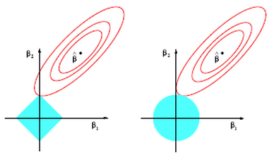
axis (in this case). The contours inscribed by the solutions (the red circles) can easily intersect the diamond at it’s tip and force \mathbf{\beta_{1}} to zero. This is much more unlikely in the case on the right for ridge regression where the \mathbf{\mathit{l}_{2}}-norm constraint inscribes a circle (in fact there is zero probability that \mathbf{\beta_{1}} will be exactly zero).

Screen Shot 2014-04-19 at 11.19.00 PM

For lasso regression, then, solutions end up looking like the graph below. As \mathbf{\lambda} increases each coefficient is eventually driven to zero.

betavloglambda

All of this begs the question, “what lambda values is ideal?” To determine this cross validation (CV) is often used. For each \mathbf{\lambda} it is possible to use CV to obtain a good estimate of the model error. You then repeat this process for all \mathbf{\lambda} within some range. The plot ends up looking like the graph below where the green line is the result of a general cross validation process and the red line uses leave-one-out cross validation. It’s interesting to note that while CV sounds like an iterative process (and in concept it is) there are fairly simple closed-form solutions for computing the CV error. I was very surprised when I first learned that! You can see below that our model should set lambda to around 4 or 5 to minimize the error (the precise value can be found by examining stored output).

CV Scores

The code to produce this graph is shown below.

# Get data
data read.csv(file = "Masked")
# Prepare data
X data[,-10]
X scale(X, center = TRUE, scale = TRUE)
response data[,10]
response scale(response, center = TRUE, scale = FALSE)
 
lambdaSeq 1:100
LOOCVscore rep(0, length(lambdaSeq))
GCVscore rep(0, length(lambdaSeq))
 
# Get leave-one-out CV score
LOOCVscore lapply(lambdaSeq,
                     FUN = function(i) {
                     lambda [i]
                     hat = X %*% (solve(t(X) %*% X + 
                     lambda*diag(ncol(X))) %*% t(X))
                     prediction = hat %*% response
                     Lii = diag(hat)
                     return(mean(((response - prediction)/
                     (1 - Lii))^2)) 
                     })
 
# Get GCV score
GCVscore lapply(lambdaSeq,
                   FUN = function(i) {
                   lambda [i]
                   hat = X %*% (solve(t(X) %*% X + 
                   lambda*diag(ncol(X))) %*% t(X))
                   prediction = hat %*% response
                   Lii = tr(hat)/nrow(X)
                   return(mean(((response - prediction)/
                   (1 - Lii))^2)) 
                   })
 
CV as.data.frame(cbind(lambdaSeq, LOOCVscore, GCVscore))
CV (CV, id = "lambdaSeq", variable_name = "CVscores")
ggplot(CV, aes(lambdaSeq, value)) + 
geom_line(aes(colour = CVscores)) +
ggtitle("A Plot of Cross Valadiation Scores vs. Lambda") + 
xlab("Lambda") + 
ylab("Cross Validation Score")

Created by Pretty R at inside-R.org

Another common statistic often presented when doing lasso regression is the shrinkage factor, which is just the ratio of the sum of the absolute value of the coefficients for the lasso solution divided by that same measure for the OLS solution. Remember small \mathbf{\lambda} forces the lasso toward the OLS solution, which implies a shrinkage factor near one should also correspond with the lasso having a solution close to OLS. You can see that patten holds below. (Code to produce this graph is shown below).

Lassobetas shrinkage

As I mentioned there is no closed-form solution that can determine the coefficients in the case of lasso regression. There are a number of methods to search through and find these betas, however. Luckily, minimizing the lasso solution results in a convex optimization problem so given enough iterations we can converge very close to the global solution. The method presented below is my implementation of the shooting algorithm. The shooting algorithm is stochastic: it picks a random beta, removes it from the model, calculates the effect of this deletion, and assigns the left out beta a value proportional to this effect, which is based on a formula I won’t present here. We were meant to determine our own criteria for stopping the loop (you could theoretically repeat this process forever). I choose a method that makes sure all betas have been updated and then calculates the MSE of the current model. If it’s within some tolerance – playing around the number suggested .001 was pretty good – the loop stops and we move on to the next lambda value. Otherwise we must continue iterating until all betas have been updated once more and the tolerance check repeats.

We were told to plot our iterations as a function of the shrinkage factor. The performance using my convergence criteria was much better than with the 1,000 iterations we were told to start with as a test case. The median number of iterations for my solution to converge quite close to the 1,000-iteration method was 103, meaning my algorithm improved performance by 10 times (at least measured by iterations).

iterationsvsConv

# Read in data
data read.csv(file = "Masked")
 
# Perpare data
X as.matrix(data[,-10])
X scale(X, center = TRUE, scale = TRUE)
response data[,10]
response scale(response, center = TRUE, scale = FALSE)
 
# Initialize variables
set.seed(35)
lambdaSeq seq(from = 1, to = 501, by = 10)
betaVectorConv matrix(NA, ncol = 7, nrow = length(lambdaSeq))
iterationsVector rep(NA, length(lambdaSeq))
aj 2*colSums(X^2)[1]
 
# Get lasso solution using shooting algorithm for each lambda
for(i in 1:length(lambdaSeq)) {
lambda [i]
betas solve(t(X) %*% X) %*% t(X) %*% response
betaUpdate rep(NA,7)
exit = FALSE
iterations  0
MSECurrent 0
MSEPast 0
 
  while(exit == FALSE) {
    j sample(1:7,1)
    betaUpdate[j] 1 
    iterations 1 
    xMinJ [,-j]
    betaMinJ [-j]
    xj [,j]
    cj 2*(t(xj) %*% (response - xMinJ %*% betaMinJ))
 
    if(cj < -lambda)      { betas[j] (cj + lambda)/aj } 
    else if(cj > lambda)  { betas[j] (cj - lambda)/aj } 
    else                  { betas[j] 0               }
 
    if(sum(is.na(betaUpdate)) == 0) {
    yHat sum((response - yHat)^2)
      if(abs(MSECurrent - MSEPast) < .001) {
      iterationsVector[i] TRUE
      }
      MSEPast rep(NA,7)
    }   
  }
  betaVectorConv[i,] }
 
#Calculate shrinkage
colnames(betaVector) colnames(X)
betaLS solve(t(X) %*% X) %*% t(X) %*% response
betaLS sum(abs(betaLS))
betaLasso abs(betaVectorConv)
betaLasso apply(betaLasso,1,sum)
betaShrink # Prepare shrinkage data for plot
betaShrinkPlot as.data.frame(cbind(betaShrink,betaVector))
betaShrinkPlot (betaShrinkPlot, id ="betaShrink",
variable_name = "betas")
 
# Plot shrinkage
ggplot(betaShrinkPlot, aes(betaShrink, value)) + 
geom_line(aes(colour = betas)) +
ggtitle("Plot of Beta Values vs. Shrinkage Factor with Conv. Crit.") + 
xlab("Shrinkage Factor") + 
ylab("Beta Value")
 
# Prepare and plot iterations
betaIterPlot as.data.frame(cbind(betaShrink, iterationsVector))
ggplot(betaIterPlot, aes(betaShrink, iterationsVector)) + 
geom_point(aes(colour = iterationsVector)) +
ggtitle("Plot of Iterations vs. Shrinkage Factor with Conv. Crit.") + 
xlab("Shrinkage Factor") + 
ylab("Iterations")

Created by Pretty R at inside-R.org

LaTeX in Stata

When doing my second HW for correlated data I came across some Stata packages that export LaTeX code directly. They are pretty similar to xTable in R. The first is the latabstat command, which is great at producing summary statistics. It outputs a LaTeX file that you can cut and paste into whatever program you are using (I use TexMakeker).  Sometimes a little additional formatting is needed, but overall it’s a much better alternative to creating LaTeX tables from scratch. Here are a few examples.

Screen Shot 2014-04-19 at 9.48.28 PM

Screen Shot 2014-04-19 at 9.48.43 PM

The second is eststo function, which is part of a separate package you have to install. It’s great for getting regression output together in a table. You can call the eststo function multiple times and then use the esttab function, which will collate all results that were prefixed with eststo. See the code below for an example use. Here are a few result tables. Again, a little modification is needed, but they look pretty good straight out of Stata.

Screen Shot 2014-04-19 at 9.48.52 PM

Screen Shot 2014-04-19 at 9.49.15 PM

Screen Shot 2014-04-19 at 9.49.24 PM


//  Load data 
C:\Users\jjmacky\Documents\Stat 540 HW 2
insheet using seizurewide.csv, clear

//  Inspect data 
br
codebook
inspect

/************ Problem 1 ************
//  Part i. 
//  Examine data by treatment status 
//  Normalize data so all variables are 
//  in terms of counts per week 
replace bl = bl/8
replace y1 = y1/2
replace y2 = y2/2
replace y3 = y3/2
replace y4 = y4/2

//  Simple table output 
tabstat y1 y2 y3 y4 bl age, by(trt) stat(n mean sd) long format ///
nototal save
latabstat y1 y2 y3 y4 bl age, by(trt) stat(mean sd) long format  ///
nototal


//  Part ii. 
//  Examine data by age 
//  Create age groups 
gen age_group = 4 if age replace age_group = 3 if age < 40
replace age_group = 2 if age < 30
replace age_group = 1 if age < 20
label define age_label 1 "Teen" 2 "Twenties" 3 "Thirties" 4 "Forties"
label values age_group age_label
//  Produce table 
tabstat bl y1 y2 y3 y4, by(age_group) stat(n mean sd) long format
latabstat bl y1 y2 y3 y4, by(age_group) stat(mean sd) long format
//  Produce graph
scatter y time, by(age_group) ytitle("Seizures per Week") xtitle("Time")

//  Part iii. 
//  Produce spaghetti plots 
//  Run this after normalizing data by seizure rate 
reshape long y, i(id) j(time)
drop if trt == 1
spagplot y time, id(id) ytitle("Seizures per Week") xtitle("Time")
//  Run this seperatly 
reshape long y, i(id) j(time)
drop if trt == 0
spagplot y time, id(id) ytitle("Seizures per Week") xtitle("Time")
//  Another possible plot 
label define trt_label 0 "Control" 1 "Treatment"
label values trt trt_label
meansdplot y time, by(trt) inner(1) ytitle("Seizures Per Week")  /// 
xtitle("Time")

//  Part B, C, D 
//  Run regressions 
//  Create variables 
gen yplus1 = y + 1
gen log_yplus1 = log(yplus1)
gen log_seizures = log(y)
gen log_age = log(age)
gen log_bl = log(bl)
//  Remove observations with no seizures (we are told to do this) 
by id (time), sort: drop if y == 0
//  Run clustered regression 
eststo: quietly regress log_seizures trt log_age log_bl, cluster(id)
//  Compare to no clustering 
eststo: quietly regress log_seizures trt log_age log_bl, robust
//  Now repeat with yplus1 as the response 
eststo: quietly regress log_yplus1 trt log_age log_bl, cluster(id)
eststo: quietly regress log_yplus1 trt log_age log_bl, robust
//  Produce Latex Result 
esttab using reg1.tex, replace


//  Part E 
//  Test effects on different times 
//  Run without reshaping 
//  Transform variables 
gen log_y1 = log(y1)
gen log_y2 = log(y2)
gen log_y3 = log(y3)
gen log_y4 = log(y4)
gen log_age = log(age)
gen log_bl = log(bl)
//  Run regressions 
eststo: quietly regress log_y1 trt log_age log_bl, cluster(id)
eststo: quietly regress log_y2 trt log_age log_bl, cluster(id)
eststo: quietly regress log_y3 trt log_age log_bl, cluster(id)
eststo: quietly regress log_y4 trt log_age log_bl, cluster(id)
//  Produce Latex Result 
esttab using reg2.tex, replace

/************ Question 2 ************/
insheet using dentalwide.csv, clear
egen numsubject = seq()
drop subject
//replace subject = numsubject 
reshape long distance, i(numsubject) j(agefrom8)
replace agefrom8 = agefrom8 - 8
gen male = cond(sex == "Male", 1, 0)

xtset numsubject agefrom8
eststo: quietly xtgee distance c.agefrom8##male, corr(independent) robust
eststo: quietly xtgee distance c.agefrom8##male, corr(exch) robust
eststo: quietly xtgee distance c.agefrom8##male, corr(ar1) robust
eststo: quietly xtgee distance c.agefrom8##male, corr(unstr) robust
esttab using gee.tex, se nostar replace

Formatted By Econometrics by Simulation

Microsoft Access

I’m learning Microsoft Access as part of a class from UW’s Information School. A lot of people are down on Microsoft, but in my opinion they usually do a good job with Office products. Access is pretty easy to learn and use and it seems powerful. It’s actually a great way to organize information even if you aren’t going to use much of the database functionality. I put some of the World Bank LSMS data I’ve been analyzing for my thesis and it’s a great way to visualize the linkages. The World Bank data has over 30 files with various one-to-one, many-to-one, and one-to-many relationships and Access seems like it would be a good platform to get a handle on the data. Although you can’ t do hardcore data analysis with Access, I think for simple data exploration using reports, queries, and forms could be quite useful.

Below are a couple of screenshots of some of the project assignments we’ve had that simulate a community college administration office.

Relations

Relationships 2