One important element of prediction and classification using regression methods is model selection. A first principle of most models is parsimony, we want to add as few predictors (explanatory variables) as is necessary to do the best we can at predicting our feature set (outcome). Often not every predictor is necessary so there is some combination that produces a balance between parsimony and accuracy.
There are simple tests to help find a model with this balance. One such test is the Akaike Information Criterion (AIC) named after the Japanese statistician Hirotugu Akaike (who was quite avuncular if his Wikipedia profile picture is any indication of his temperament). In math speak, the AIC maximizes the likelihood function by using convex optimization and has an added penalty as more predictors are added to the model.
There are simple ways to select a model. One easy way is to try every possible combination of predictors and see which one has the best AIC. At some point adding additional predictors will fail to produce much improvement in predicting the feature set and we know we can stop. This is pretty easy if you have five or ten predictor, but the number of models to test grows exponentially.
For example, a recent dataset we were given for homework in a graduate statistics course I’m taking, included 60 predictors. Each predictor can be either added to the model or left out resulting in  (
( ) possible models (including the null model with only the intercept). To give a sense of how large that is, it’s beginning to approach the number of starts in the observable universe (
 ). Even modern computers would take too long to test every possible model.
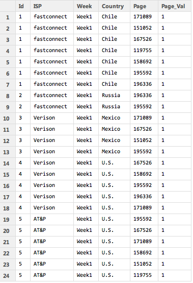
And some models have even more variables. Many more. High-dimensional models with thousands of predictors are not uncommon. One popular example in machine learning uses MRI images where each pixel (called a voxel in this setting because it represents a 3-D slice of the brain) represents a predictor. Here there are 20,000 possible predictors: each voxel of the image can be in or out of the model, representing weather that part of the brain is important in predicting some neurologic outcome. (In practice particular – as common sense would imply – there is some dependency in choosing voxels, which makes the task slightly different).
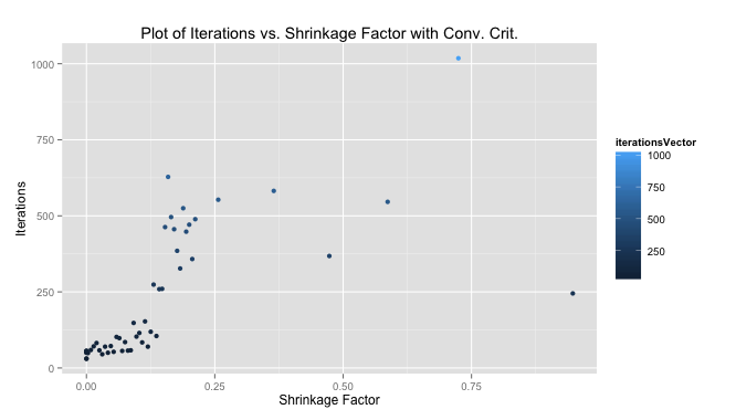
One alternative to testing every possible combination of predictors is using a Markov Chain Monte Carlo Model Composition(MC3). It’s just a fancy way of saying that we choose a model at random and then move randomly (but intelligently) toward models that have a better AIC score.
We were asked to implement such an algorithm recently for my class. It was a pretty fun project that took some creative thinking to make efficient. The MC3 algorithm is pretty simple. We pick a random model with a random number of predictors. Then we look at all of the valid models that leave one of these predictors out as well as the valid models that add one predictor. This is called the “neighborhood” of the model. We choose one of these new models in the neighborhood at random and compute a modified version of the AIC. If it’s better than our current model’s AIC we move to that model and repeat the process. Otherwise we randomly select another candidate model, compute it’s AIC, compare scores to the current model and repeat until we move to a new model.
We were given several starter functions by our professor. All three are pretty trivial to implement oneself aside from isValidLogisticRCDD(), which implements a model validity test from a statistics paper using deep theoretical concepts far beyond mathematical knowledge.
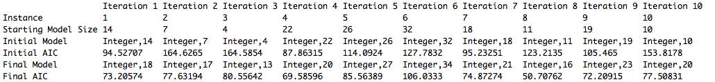
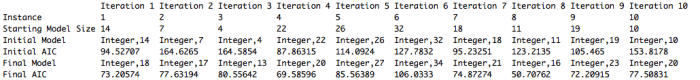
My results are shown below. We were meant to run the algorithm for 10 instances of 25 iterations each. I store all of the relevant information in a list so when the algorithm is done running I get a nice little output. I just realize the “Iteration [number]” at the top of each column should really say “Instance”. Oops!! Just went back and fixed that in my code.
The R code is shown below. It looks a little funky because we are transitioning to writing in C and our professor wants us to start getting into the C mindset. I’m also trying to write more loops using the apply() function instead of the traditional for loop. There are all kinds of debates online about under what cases apply() is faster than a for loop and if it’s even true in general anymore. At any rate it’s good to familiarize myself with different techniques and look at problems in different ways. I wrote several helper functions to find a models neighborhood and test the valid members in it. The MC3 function appears near the bottom along with a main() function.
#######################################################
# James McCammon
# Description:
# MC3 uses several custom helper functions to determine
# the best AIC of a model using a markov chain process.
#######################################################


#######################################################
# Given Functions
#######################################################
getLogisticAIC <- function(response,explanatory,data)
isValidLogistic <- function(response,explanatory,data)
isValidLogisticRCDD <- function(response,explanatory,data)


##########################################################
# Custom Functions
##########################################################

############### checkModelValidity Function ###############
# Checks if a particular model is valid by first doing
# preliminary empirical test and then moving on to a more
# robust theoretical test
checkModelValidity <- function(response,explanatory,data) {
  prelimCheck <- isValidLogistic(response,explanatory,data)
  if(!prelimCheck) { return(FALSE) }
  robustCheck <- isValidLogisticRCDD(response,explanatory,data)
  if(!robustCheck) { return(FALSE) }
  return(TRUE)
}

############### findNeighboursBelow Function ###############
# Given an arbitrary vector this function finds the set of
# all vectors generated by leaving one element out.
findNeighboursBelow  <- function(elements) {
  if(is.null(elements)) { return(NULL) }
  length = length(elements);
  neighbours = vector("list",length);
  neighbours = lapply(1:length,
                      FUN = function(i) {
                      return(elements[-i])
                      })
  return(neighbours);
}

############### findNeighboursAbove Function ###############
# Given an arbitrary vector this function finds the set of
# all vectors generated by adding an element not already in
# the set given an upper bound of possible elements to add.
findNeighboursAbove <- function(elements, last) {
  fullModel = seq(1,last);
  notInModel = setdiff(fullModel,elements);
  length = length(notInModel);
  neighbours = vector("list",length);
  neighbours = lapply(1:length,
                      FUN = function(i) {
                      return(union(elements, notInModel[i]))
                      })
  return(neighbours);
}

############### findValidNeighboursAbove Function ###############
# This function finds all of the valid neighbouring models produced
# by using the findNeighboursAbove function.
findValidNeighboursAbove <- function(response, explanatory, last, data) {
  neighbours = findNeighboursAbove(explanatory,last);
  length = length(neighbours);
  keep = rep(NA, length);
  keep = lapply(1:length,
                FUN = function(i) {
                return(checkModelValidity(response,
                neighbors[[i]], data))
                })
  validNeighboursAbove = neighbours[as.logical(keep)];
  return(validNeighboursAbove);
}

##########################################################
# MC3 Function
##########################################################

MC3 <- function(response, explanatory, iterations, instances,
lastPredictor) {
  require(rcdd);
  finalResults = NULL

  for(k in 1:instances) {
    # Make sure you start with a valid model
    initialModelValid = FALSE;
    while(!initialModelValid) {
      modelSize = sample(explanatory,1);
      initialModel = sample(explanatory, modelSize);
      initialModelValid = checkModelValidity(response, initialModel,      data);
    }

    # Get measures for initial model
    currentModel = initialModel;
    currentAIC = getLogisticAIC(response,currentModel,data);

    # Check to see if we should start at the null model
    nullModelAIC = getLogisticAIC(response = response, explanatory =    NULL, data = data)
    if(nullModelAIC < currentAIC) {
      currentModel = NULL;
      currentAIC = nullModelAIC;
      initialModel = NULL;
    }

    # Store initial AIC for later output.
    initialModel = currentModel;
    initialAIC = currentAIC;

    # Get valid neighbors of current model
    currValidNeighAbove = findValidNeighboursAbove(response,
    currentModel, lastPredictor, data);
    currValidNeighBelow = findNeighboursBelow(currentModel);
    currAllNeigh = c(currValidNeighAbove, currValidNeighBelow);
    # Compute score
    currentScore = -currentAIC - log(length(currAllNeigh));

    # Iterate for the number of times specified.
    for(i in 1:iterations) {
      # Compute measures for the candidate model
      candidateIndex = sample(1:length(currAllNeigh),1);
      candidateModel = currAllNeigh[[candidateIndex]];
      candValidNeighAbove = findValidNeighboursAbove(response,
      candidateModel, lastPredictor, data);
      candValidNeighBelow = findNeighboursBelow(candidateModel);
      candAllNeigh = c(candValidNeighAbove, candValidNeighBelow);

      candidateAIC = getLogisticAIC(response, candidateModel, data);
      candidateScore = -candidateAIC - log(length(candAllNeigh));

      # If necessary move to the candidate model.
      if(candidateScore > currentScore) {
        currentModel = candidateModel;
        currAllNeigh = candAllNeigh;
        currentAIC = candidateAIC;
        currentScore = candidateScore;
      }
      # Print results as we iterate.
      print(paste('AIC on iteration', i ,'of instance', k , 'is',
      round(currentAIC,2)));
    }

    # Produce outputs
    instanceResults = (list(
                       "Instance"            = k,
                       "Starting Model Size" = modelSize,
                       "Initial Model"       = sort(initialModel),
                       "Initial AIC"         = initialAIC,
                       "Final Model"         = sort(currentModel),
                       "Final AIC"           = currentAIC));
    finalResults = cbind(finalResults, instanceResults);
    colnames(finalResults)[k] = paste("Instance",k)
  }
  return(finalResults);
}

##########################################################
# Main Function
##########################################################

main <- function(data, iterations, instances) {
  response = ncol(data);
  lastPredictor = ncol(data)-1;
  explanatory = 1:lastPredictor;
  results = MC3(response, explanatory, iterations, instances,
  lastPredictor);
  return(results);
}

##########################################################
# Run Main
##########################################################
setwd("~/Desktop/Classes/Stat 534/Assignment 3")
data = as.matrix(read.table(file = "534binarydata.txt", header =
FALSE));
main(data, iterations = 25, instances = 10);
Created by Pretty R at inside-R.org
We were meant to run 10 instances of the algorithm for 25 iterations each. My best run was instance 8. I print out the AIC at every iteration to help keep track of things and give me that nice reassurance that R isn’t exploding at the sight of my code, which is always a fear when nothing is output for more than 5 minutes.
[1] "AIC on iteration 1 of instance 8 is 123.21"
[1] "AIC on iteration 2 of instance 8 is 104.17"
[1] "AIC on iteration 3 of instance 8 is 104.17"
[1] "AIC on iteration 4 of instance 8 is 97.31"
[1] "AIC on iteration 5 of instance 8 is 88.52"
[1] "AIC on iteration 6 of instance 8 is 88.25"
[1] "AIC on iteration 7 of instance 8 is 88.25"
[1] "AIC on iteration 8 of instance 8 is 86.64"
[1] "AIC on iteration 9 of instance 8 is 86.64"
[1] "AIC on iteration 10 of instance 8 is 83.67"
[1] "AIC on iteration 11 of instance 8 is 83.67"
[1] "AIC on iteration 12 of instance 8 is 83.67"
[1] "AIC on iteration 13 of instance 8 is 81.77"
[1] "AIC on iteration 14 of instance 8 is 81.77"
[1] "AIC on iteration 15 of instance 8 is 56.96"
[1] "AIC on iteration 16 of instance 8 is 56.96"
[1] "AIC on iteration 17 of instance 8 is 54.45"
[1] "AIC on iteration 18 of instance 8 is 54.45"
[1] "AIC on iteration 19 of instance 8 is 52.69"
[1] "AIC on iteration 20 of instance 8 is 52.69"
[1] "AIC on iteration 21 of instance 8 is 52.69"
[1] "AIC on iteration 22 of instance 8 is 50.71"
[1] "AIC on iteration 23 of instance 8 is 50.71"
[1] "AIC on iteration 24 of instance 8 is 50.71"
[1] "AIC on iteration 25 of instance 8 is 50.71"
Created by Pretty R at inside-R.org


 -norm while lasso regression uses the
  -norm. Specifically the forms are shown below.

 The only difference is the
  term. I read (or heard) somewhere that ridge regression was originally designed to deal with invertability issues in OLS. By adding the small
  is close to zero the ridge solution approachese the least squares solution. As
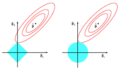
 axis (in this case). The contours inscribed by the solutions (the red circles) can easily intersect the diamond at it’s tip and force
  to zero. This is much more unlikely in the case on the right for ridge regression where the