Lasso and ridge regression are two alternatives – or should I say complements – to ordinary least squares (OLS). They both start with the standard OLS form and add a penalty for model complexity. The only difference between the two methods is the form of the penality term. Ridge regression uses the -norm while lasso regression uses the -norm. Specifically the forms are shown below.

Ridge Regression:

Lasso Regression:

Ridge regression has a closed form solution that is quite similar to that of OLS: The only difference is the term. I read (or heard) somewhere that ridge regression was originally designed to deal with invertability issues in OLS. By adding the small  term we get the inner product to move away from possible singular matrices.

In ridge regreession when is close to zero the ridge solution approachese the least squares solution. As increases the solutions are forced toward zero. You can see this behavior graphed below for a sample dataset.

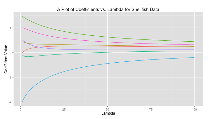
The code to produce this graph is quite simple.

# Load libraries
library(MASS)
library(reshape)
library(psych)
library(ggplot2)
 
# Get data
data read.csv(file = "Masked")
# Prepare data
X data[,-10]
X scale(X, center = TRUE, scale = TRUE)
response data[,10]
response scale(reponse, center = TRUE, scale = FALSE)
 
# Get ridge solution for every lambda
betas matrix(rep(NA), nrow = 7, ncol = 100)
rownames(betas) colnames(X)
lambda 1:100
betas lapply(1:length(lambda),
               FUN = function(i) {  
               return(solve(t(X)%*%X + diag(x = lambda[i], 
               ncol(X)) )%*%t(X)%*%response)  
               })
 
# Prepare data for plot
betas data.frame(t(betas))
betas cbind(lambda, betas)
betas (betas, id = "lambda", variable_name = "coviariate")
 
# Plot
ggplot(betas, aes(lambda, value)) + 
geom_line(aes(colour = coviariate)) + 
ggtitle("A Plot of Coefficients vs. Lambda for Shellfish Data") + 
xlab("Lambda") + 
ylab("Coefficient Value") + 
theme(legend.position = "none")

Lasso on the other hand does not have a closed form solution so numerical techniques are required. The benefit of lasso, however, is that coefficients are driven to exactly zero. In this way lasso acts as a sort of model selection process. The reason ridge regression solutions do not hit exactly zero, but lasso solutions do is because of the differing nature of the geometry of the -norm and -norm. In two dimensions the difference can be viewed in the picture below. Lasso regression constraints make a diamond aligned with the axis (in this case). The contours inscribed by the solutions (the red circles) can easily intersect the diamond at it’s tip and force  to zero. This is much more unlikely in the case on the right for ridge regression where the -norm constraint inscribes a circle (in fact there is zero probability that  will be exactly zero).

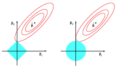
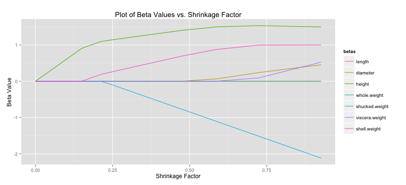
For lasso regression, then, solutions end up looking like the graph below. As  increases each coefficient is eventually driven to zero.

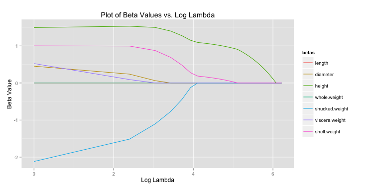
All of this begs the question, “what lambda values is ideal?” To determine this cross validation (CV) is often used. For each  it is possible to use CV to obtain a good estimate of the model error. You then repeat this process for all  within some range. The plot ends up looking like the graph below where the green line is the result of a general cross validation process and the red line uses leave-one-out cross validation. It’s interesting to note that while CV sounds like an iterative process (and in concept it is) there are fairly simple closed-form solutions for computing the CV error. I was very surprised when I first learned that! You can see below that our model should set lambda to around 4 or 5 to minimize the error (the precise value can be found by examining stored output).

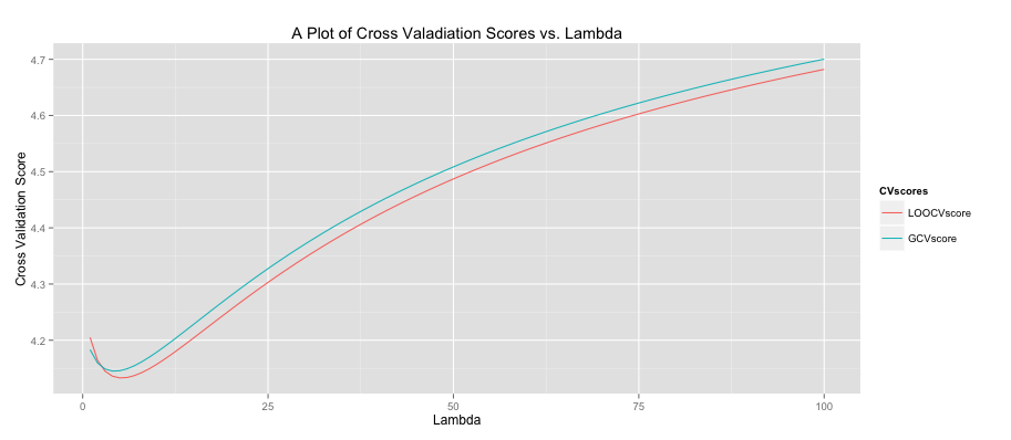
The code to produce this graph is shown below.

# Get data
data read.csv(file = "Masked")
# Prepare data
X data[,-10]
X scale(X, center = TRUE, scale = TRUE)
response data[,10]
response scale(response, center = TRUE, scale = FALSE)
 
lambdaSeq 1:100
LOOCVscore rep(0, length(lambdaSeq))
GCVscore rep(0, length(lambdaSeq))
 
# Get leave-one-out CV score
LOOCVscore lapply(lambdaSeq,
                     FUN = function(i) {
                     lambda [i]
                     hat = X %*% (solve(t(X) %*% X + 
                     lambda*diag(ncol(X))) %*% t(X))
                     prediction = hat %*% response
                     Lii = diag(hat)
                     return(mean(((response - prediction)/
                     (1 - Lii))^2)) 
                     })
 
# Get GCV score
GCVscore lapply(lambdaSeq,
                   FUN = function(i) {
                   lambda [i]
                   hat = X %*% (solve(t(X) %*% X + 
                   lambda*diag(ncol(X))) %*% t(X))
                   prediction = hat %*% response
                   Lii = tr(hat)/nrow(X)
                   return(mean(((response - prediction)/
                   (1 - Lii))^2)) 
                   })
 
CV as.data.frame(cbind(lambdaSeq, LOOCVscore, GCVscore))
CV (CV, id = "lambdaSeq", variable_name = "CVscores")
ggplot(CV, aes(lambdaSeq, value)) + 
geom_line(aes(colour = CVscores)) +
ggtitle("A Plot of Cross Valadiation Scores vs. Lambda") + 
xlab("Lambda") + 
ylab("Cross Validation Score")

Created by Pretty R at inside-R.org

Another common statistic often presented when doing lasso regression is the shrinkage factor, which is just the ratio of the sum of the absolute value of the coefficients for the lasso solution divided by that same measure for the OLS solution. Remember small  forces the lasso toward the OLS solution, which implies a shrinkage factor near one should also correspond with the lasso having a solution close to OLS. You can see that patten holds below. (Code to produce this graph is shown below).

As I mentioned there is no closed-form solution that can determine the coefficients in the case of lasso regression. There are a number of methods to search through and find these betas, however. Luckily, minimizing the lasso solution results in a convex optimization problem so given enough iterations we can converge very close to the global solution. The method presented below is my implementation of the shooting algorithm. The shooting algorithm is stochastic: it picks a random beta, removes it from the model, calculates the effect of this deletion, and assigns the left out beta a value proportional to this effect, which is based on a formula I won’t present here. We were meant to determine our own criteria for stopping the loop (you could theoretically repeat this process forever). I choose a method that makes sure all betas have been updated and then calculates the MSE of the current model. If it’s within some tolerance – playing around the number suggested .001 was pretty good – the loop stops and we move on to the next lambda value. Otherwise we must continue iterating until all betas have been updated once more and the tolerance check repeats.

We were told to plot our iterations as a function of the shrinkage factor. The performance using my convergence criteria was much better than with the 1,000 iterations we were told to start with as a test case. The median number of iterations for my solution to converge quite close to the 1,000-iteration method was 103, meaning my algorithm improved performance by 10 times (at least measured by iterations).

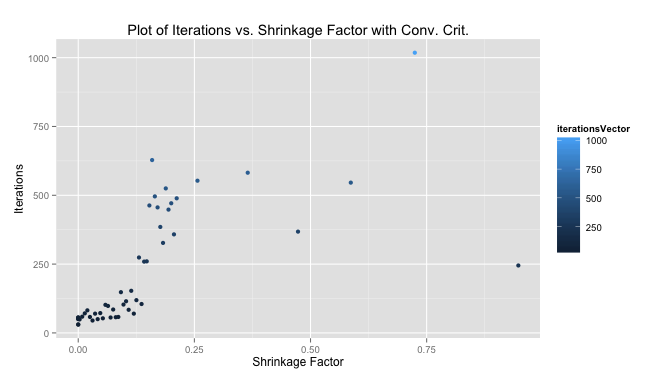
# Read in data
data read.csv(file = "Masked")
 
# Perpare data
X as.matrix(data[,-10])
X scale(X, center = TRUE, scale = TRUE)
response data[,10]
response scale(response, center = TRUE, scale = FALSE)
 
# Initialize variables
set.seed(35)
lambdaSeq seq(from = 1, to = 501, by = 10)
betaVectorConv matrix(NA, ncol = 7, nrow = length(lambdaSeq))
iterationsVector rep(NA, length(lambdaSeq))
aj 2*colSums(X^2)[1]
 
# Get lasso solution using shooting algorithm for each lambda
for(i in 1:length(lambdaSeq)) {
lambda [i]
betas solve(t(X) %*% X) %*% t(X) %*% response
betaUpdate rep(NA,7)
exit = FALSE
iterations  0
MSECurrent 0
MSEPast 0
 
  while(exit == FALSE) {
    j sample(1:7,1)
    betaUpdate[j] 1 
    iterations 1 
    xMinJ [,-j]
    betaMinJ [-j]
    xj [,j]
    cj 2*(t(xj) %*% (response - xMinJ %*% betaMinJ))
 
    if(cj < -lambda)      { betas[j] (cj + lambda)/aj } 
    else if(cj > lambda)  { betas[j] (cj - lambda)/aj } 
    else                  { betas[j] 0               }
 
    if(sum(is.na(betaUpdate)) == 0) {
    yHat sum((response - yHat)^2)
      if(abs(MSECurrent - MSEPast) < .001) {
      iterationsVector[i] TRUE
      }
      MSEPast rep(NA,7)
    }   
  }
  betaVectorConv[i,] }
 
#Calculate shrinkage
colnames(betaVector) colnames(X)
betaLS solve(t(X) %*% X) %*% t(X) %*% response
betaLS sum(abs(betaLS))
betaLasso abs(betaVectorConv)
betaLasso apply(betaLasso,1,sum)
betaShrink # Prepare shrinkage data for plot
betaShrinkPlot as.data.frame(cbind(betaShrink,betaVector))
betaShrinkPlot (betaShrinkPlot, id ="betaShrink",
variable_name = "betas")
 
# Plot shrinkage
ggplot(betaShrinkPlot, aes(betaShrink, value)) + 
geom_line(aes(colour = betas)) +
ggtitle("Plot of Beta Values vs. Shrinkage Factor with Conv. Crit.") + 
xlab("Shrinkage Factor") + 
ylab("Beta Value")
 
# Prepare and plot iterations
betaIterPlot as.data.frame(cbind(betaShrink, iterationsVector))
ggplot(betaIterPlot, aes(betaShrink, iterationsVector)) + 
geom_point(aes(colour = iterationsVector)) +
ggtitle("Plot of Iterations vs. Shrinkage Factor with Conv. Crit.") + 
xlab("Shrinkage Factor") + 
ylab("Iterations")

Created by Pretty R at inside-R.org