Suppose we consider a simple random walk. A particle starts at initial position 


![\mathbb{E}[X_n]](https://s0.wp.com/latex.php?latex=%5Cmathbb%7BE%7D%5BX_n%5D+&bg=ffffff&fg=000000&s=0&c=20201002)

In a previous post I presented a method to solve this by iteration. I’d like to present a different method to solve the problem here.
Recall we have:
We give it some thought we can see that after

So now all we need to do is take the expected value of 

![\mathbb{E}[Y] = \mathbb{E}\big[\sum_{i=1}^{n} X_i \big]](https://s0.wp.com/latex.php?latex=%5Cmathbb%7BE%7D%5BY%5D+%3D+%5Cmathbb%7BE%7D%5Cbig%5B%5Csum_%7Bi%3D1%7D%5E%7Bn%7D+X_i+%5Cbig%5D+&bg=ffffff&fg=000000&s=0&c=20201002)
![\mathbb{E}[Y] = \sum_{i=1}^{n} \mathbb{E}[X_i]](https://s0.wp.com/latex.php?latex=%5Cmathbb%7BE%7D%5BY%5D+%3D+%5Csum_%7Bi%3D1%7D%5E%7Bn%7D+%5Cmathbb%7BE%7D%5BX_i%5D+&bg=ffffff&fg=000000&s=0&c=20201002)
![\mathbb{E}[Y] = \sum_{i=1}^{n} -1 \cdot p + 1 \cdot (1-p)](https://s0.wp.com/latex.php?latex=%5Cmathbb%7BE%7D%5BY%5D+%3D%C2%A0%5Csum_%7Bi%3D1%7D%5E%7Bn%7D+-1+%5Ccdot+p+%2B+1+%5Ccdot+%281-p%29+&bg=ffffff&fg=000000&s=0&c=20201002)
![\mathbb{E}[Y] = \sum_{i=1}^{n} 1 - 2p](https://s0.wp.com/latex.php?latex=%5Cmathbb%7BE%7D%5BY%5D+%3D+%C2%A0%5Csum_%7Bi%3D1%7D%5E%7Bn%7D+1+-+2p+&bg=ffffff&fg=000000&s=0&c=20201002)
![\mathbb{E}[Y] = n(1 - 2p)](https://s0.wp.com/latex.php?latex=%5Cmathbb%7BE%7D%5BY%5D+%3D+n%281+-+2p%29+&bg=ffffff&fg=000000&s=0&c=20201002)
This is the same answer we got via the iteration method. This also makes our R simulation easier. Recall we has this setup:
################################################################
# R Simulation
################################################################
# Generate random walk
rand_walk = function (n, p, z) {
  walk = sample(c(-1,1), size=n, replace=TRUE, prob=c(p,1-p))
  for (i in 1:n) {
    z = z + walk[i]
  }
  return(z)
}

n = 1000 # Walk n steps
p = .3 # Probability of moving left
z = 0 # Set initial position to 0
trials = 10000 # Num times to repeate sim
# Run simulation
X = replicate(trials, rand_walk(n,p,z))
Our code now becomes:
################################################################
# R Simulation
################################################################
n = 1000 # Walk n steps
p = .3 # Probability of moving left
trials = 10000 # Num times to repeate sim
# Run simulation
X = replicate(trials, sum(sample(c(-1,1), size=n, replace=TRUE, prob=c(p,1-p))))

# Calculate empirical and theoretical results
empirical = mean(X)
theoretical = n*(1-2*p)
percent_diff = abs((empirical-theoretical)/empirical)*100

# print to console
empirical
theoretical
percent_diff
Notice that for our random walk we can replace this function:
rand_walk = function (n, p, z) {
  walk = sample(c(-1,1), size=n, replace=TRUE, prob=c(p,1-p))
  for (i in 1:n) {
    z = z + walk[i]
  }
  return(z)
}
X = replicate(trials, rand_walk(n,p,z))
With the simpler:
X = replicate(trials, sum(sample(c(-1,1), size=n, replace=TRUE, prob=c(p,1-p))))
Additionally, in this second method we don’t need to specify an initial position since we assume from the beginning it’s zero. Of course both methods complete the same task, but they use different conceptual models. The first uses an iteration model, while the latter completes the “iteration” in a single step.
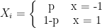
 for
for  ,
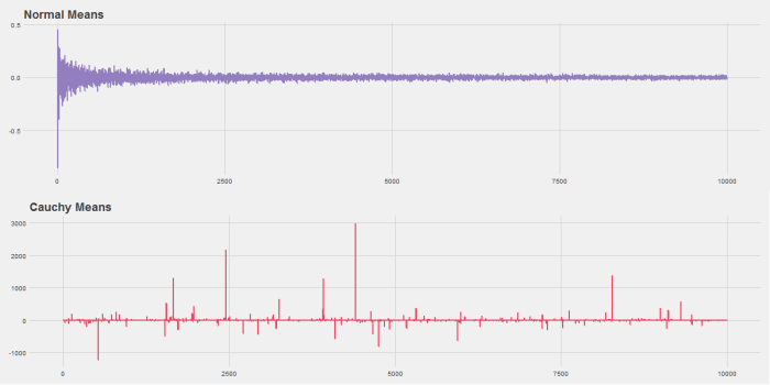
,  . Suppose we want to do the same for the Cauchy distribution.