Suppose we want to simulate  for
for  ,
,  . Suppose we want to do the same for the Cauchy distribution.
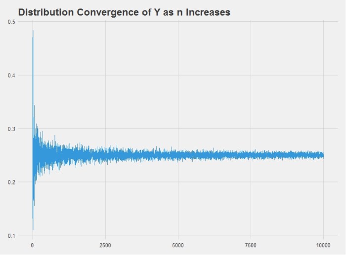
In other words, we want to draw several random variables from a normal distribution and then take the average. As  increases we should get closer to the mean of the distribution we’re drawing from, 0 in this case.
The R code below will do this. It produces this graph:
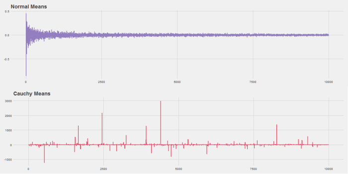
Notice that while the Normal distribution converges quickly the Cauchy never does. This is because the Cauchy distribution has fat tails and so extreme observations are common.
################################################################
# R Simulation
# James McCammon
# 2/20/2017
################################################################
# This script goes through the simulation of plotting both normal
# and Cauchy means for random vectors of size 1 to 10,000. It
# also demonstrates function creation and plotting.
# Highlight desired section and click "Run."

# Set working directory as needed
setwd("~/R Projects/All of Statistics")

###
# Calculate means and plot using base R
###

    # Set seed for reproducibility
    set.seed(271)

    #
    # Version 1: Simple
    #
    n = seq(from=1, to=10000, by=1)
    y=sapply(n, FUN=function(x) sum(rnorm(x))/x)
    plot(n, y, type="l")

    #
    # Version 2: Define a function
    #
    sim = function(x, FUN) {
      sapply(x, FUN=function(x) sum(FUN(x))/x)
    }

    # Use function to plot normal means
    x = seq(from=1, to=10000, by=1)
    y1 = sim(x, rnorm)
    plot(x, y1, type="l")

    # Use function to plot Cauchy means
    y2 = sim(x, rcauchy)
    plot(x, y2, type="l")

    #
    # Version 3: More complex function
    #

    # This function has:
    # (1) error checking
    # (2) extra argument options
    # (3) the ability to input any distribution R supports
    sim = function(x, FUN, ...) {
      if(!is.character(FUN)) stop('Please enter distribution as string.')
      dists = c('rnorm',
                'rbeta',
                'rbinom',
                'rcauchy',
                'rchisq',
                'rexp',
                'rf',
                'rgamma',
                'rgeom',
                'rhyper',
                'rlnorm',
                'rmultinom',
                'rnbinom',
                'rpois',
                'rt',
                'runif',
                'rweibull')
      if(is.na(match(FUN, dists))) stop(paste('Please enter a valid distribution from one of:', paste(dists, collapse=', ')))
      FUN = get(FUN)
      sapply(x, FUN=function(x) sum(FUN(x, ...))/x)
    }

    # We have to define our function in string form.
    # This will throw error 1.
    test1 = sim(x, rnorm)

    # We have to input a distribution R supports.
    # This will throw error 2.
    test2 = sim(x, 'my_cool_function')

    # We can input additional arguments like the
    # mean, standard deviations, or other shape parameters.
    test3 = sim(x, 'rnorm', mean=10, sd=2)

####
# Using ggplot2 to make pretty graph
###

    # Load libraries
    library(ggplot2)
    library(ggthemes)
    library(gridExtra)

    png(filename='Ch3-Pr9.png', width=1200, height=600)

      df1 = cbind.data.frame(x, y1)
      p1 = ggplot(df1, aes(x=x, y=y1)) +
        geom_line(size = 1, color='#937EBF') +
        theme_fivethirtyeight() +
        ggtitle("Normal Means")

      df2 = cbind.data.frame(x, y2)
      p2 = ggplot(df2, aes(x=x, y=y2)) +
        geom_line(size = 1, color='#EF4664') +
        theme_fivethirtyeight() +
        ggtitle("Cauchy Means")

      # Save charts
      grid.arrange(p1,p2,nrow=2,ncol=1)

    dev.off()
    # Print charts to screen
    grid.arrange(p1,p2,nrow=2,ncol=1)


![\bar{X}_n \overset{P}{\longrightarrow} \mathbb{E}[X]](https://s0.wp.com/latex.php?latex=%5Cbar%7BX%7D_n+%5Coverset%7BP%7D%7B%5Clongrightarrow%7D+%5Cmathbb%7BE%7D%5BX%5D+&bg=ffffff&fg=000000&s=0&c=20201002)

![\mathbb{E}[X] = .5](https://s0.wp.com/latex.php?latex=%5Cmathbb%7BE%7D%5BX%5D+%3D+.5+&bg=ffffff&fg=000000&s=0&c=20201002)
![Y_n \rightsquigarrow \mathbb{E}[X]\mathbb{E}[X]](https://s0.wp.com/latex.php?latex=Y_n+%5Crightsquigarrow+%5Cmathbb%7BE%7D%5BX%5D%5Cmathbb%7BE%7D%5BX%5D+&bg=ffffff&fg=000000&s=0&c=20201002)