My friend Ryan, who is also a math tutor at UW, and I are working our way through several math resources including Larry Wasserman’s famous All of Statistics. Here is a math problem:
Suppose we have  random variables
  all distributed uniformly,
  . We want to find the expected value of
 ![\mathbb{E}[Y_n]](https://s0.wp.com/latex.php?latex=%5Cmathbb%7BE%7D%5BY_n%5D+&bg=ffffff&fg=000000&s=0&c=20201002) where
where  .
.
First, we need to find the Probability Density Function (PDF)  and we do so in the usual way, by first finding the Cumulative Distribution Function (CDF) and taking the derivative:


We want to be able to get this step:

But must show independence and we are not give that our  ‘s are in fact independent. Thanks to Ryan for helping me see that by definition:

However, note that in this case  is a unit
  with area
  equal to
  . In other words
  . Our equation then simplifies:

![F_Y(y) = \int dx_1 \dots \int dx_n = [F_X(y)]^n](https://s0.wp.com/latex.php?latex=F_Y%28y%29+%3D+%5Cint+dx_1+%5Cdots+%5Cint+dx_n+%3D+%5BF_X%28y%29%5D%5En+&bg=ffffff&fg=000000&s=0&c=20201002) where
where  here is a generic random variable, by symmetry (all ‘s are identically distributed). This is the same answer we would’ve gotten if we made the iid assumption earlier and obtained . Originally, I had made this assumption by way of wishful thinking — and a bit of intuition, it does seem that uniformly distributed random variables would be independent — but Ryan corrected my mistake.
Now that we have  we can find the PDF.
![f_Y(y) = \frac{d}{dy}F_Y(y) = \frac{d}{dy}[F_X(y)]^n](https://s0.wp.com/latex.php?latex=f_Y%28y%29+%3D+%5Cfrac%7Bd%7D%7Bdy%7DF_Y%28y%29+%3D+%5Cfrac%7Bd%7D%7Bdy%7D%5BF_X%28y%29%5D%5En+&bg=ffffff&fg=000000&s=0&c=20201002)
![f_Y(y) = n[F_X(y)]^{n-1}f_X(y)](https://s0.wp.com/latex.php?latex=f_Y%28y%29+%3D+n%5BF_X%28y%29%5D%5E%7Bn-1%7Df_X%28y%29+&bg=ffffff&fg=000000&s=0&c=20201002) by the chain rule.
by the chain rule.
Recall that the PDF  of a
of a  is
is  for
for ![x \in [0,1]](https://s0.wp.com/latex.php?latex=x+%5Cin+%5B0%2C1%5D+&bg=ffffff&fg=000000&s=0&c=20201002) . And by extension the CDF
. And by extension the CDF  for a is:
 .
.
Plugging these values into our equation above (and noting we have  not
not  meaning we simply replace the
  we just derived with
  as we would in any normal function) we have:
Finally, we are ready to take our expectation:
![\mathbb{E}[Y] = \int_{y\in A}yf_Y(y)dy = \int_0^1 yny^{n-1}dy = n\int_0^1 y^{n}dy = n\bigg[\frac{1}{n+1}y^{n+1}\bigg]_0^1 = \frac{n}{n+1}](https://s0.wp.com/latex.php?latex=%5Cmathbb%7BE%7D%5BY%5D+%3D+%5Cint_%7By%5Cin+A%7Dyf_Y%28y%29dy+%3D+%5Cint_0%5E1+yny%5E%7Bn-1%7Ddy+%3D+n%5Cint_0%5E1+y%5E%7Bn%7Ddy+%3D+n%5Cbigg%5B%5Cfrac%7B1%7D%7Bn%2B1%7Dy%5E%7Bn%2B1%7D%5Cbigg%5D_0%5E1+%3D+%5Cfrac%7Bn%7D%7Bn%2B1%7D&bg=ffffff&fg=000000&s=0&c=20201002)
Let’s take a moment and make sure this answer seems reasonable. First, note that if we have the trival case of  (which is simply
  ;
;  in this case) we get
  . This makes sense! If then
  is just a uniform random variable on the interval
  to . And the expected value of that random variable is
  which is exactly what we got.
Also notice that  . This also makes sense! If we take the maximum of 1 or 2 or 3 ‘s each randomly drawn from the interval 0 to 1, we would expect the largest of them to be a bit above , the expected value for a single uniform random variable, but we wouldn’t expect to get values that are extremely close to 1 like .9. However, if we took the maximum of, say, 100 ‘s we would expect that at least one of them is going to be pretty close to 1 (and since we’re choosing the maximum that’s the one we would select). This doesn’t guarantee our math is correct (although it is), but it does give a gut check that what we derived is reasonable.
We can further verify our answer by simulation in R, for example by choosing  (thanks to the fantastic Markup.su syntax highlighter):
################################################################
# R Simulation
################################################################
X = 5
Y = replicate(100000, max(runif(X)))
empirical = mean(Y)
theoretical = (X/(X+1)) #5/6 = 8.33 in this case
percent_diff = abs((empirical-theoretical)/empirical)*100

# print to console
empirical
theoretical
percent_diff
We can see from our results that our theoretical and empirical results differ by just 0.05% after 100,000 runs of our simulation.
> empirical
[1] 0.8337853
> theoretical
[1] 0.8333333
> percent_diff
[1] 0.0542087

 and are given that
 ![\lim_{n\to\infty} x\big[1-F(x)\big] = 0](https://s0.wp.com/latex.php?latex=%5Clim_%7Bn%5Cto%5Cinfty%7D+x%5Cbig%5B1-F%28x%29%5Cbig%5D+%3D+0+&bg=ffffff&fg=000000&s=0&c=20201002) . Show that
. Show that ![\mathbb{E}[X] = \int_0^{\infty} P(X > x)dx](https://s0.wp.com/latex.php?latex=%5Cmathbb%7BE%7D%5BX%5D+%3D+%5Cint_0%5E%7B%5Cinfty%7D+P%28X+%3E+x%29dx+&bg=ffffff&fg=000000&s=0&c=20201002) .
.![\mathbb{E}[X] = \int_{-\infty}^{\infty}xf_X(x)dx = \int_0^{\infty}xf_X(x)dx](https://s0.wp.com/latex.php?latex=%5Cmathbb%7BE%7D%5BX%5D+%3D+%5Cint_%7B-%5Cinfty%7D%5E%7B%5Cinfty%7Dxf_X%28x%29dx+%3D+%5Cint_0%5E%7B%5Cinfty%7Dxf_X%28x%29dx&bg=ffffff&fg=000000&s=0&c=20201002) since we are given
since we are given  .
.
 and plugging in our selections we get:
![\mathbb{E}[X] = \int_0^{\infty}xf_X(x)dx = xF_X(x)\bigm|_0^{\infty} - \int_0^{\infty} F_X(x)dx](https://s0.wp.com/latex.php?latex=%5Cmathbb%7BE%7D%5BX%5D+%3D+%5Cint_0%5E%7B%5Cinfty%7Dxf_X%28x%29dx+%3D+xF_X%28x%29%5Cbigm%7C_0%5E%7B%5Cinfty%7D+-+%5Cint_0%5E%7B%5Cinfty%7D+F_X%28x%29dx+&bg=ffffff&fg=000000&s=0&c=20201002)
 as
as 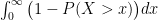 . This simplifies to
 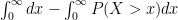 . Let’s plug this back into our equation above:
![\mathbb{E}[X] = \int_0^{\infty}xf_X(x)dx = xF_X(x)\bigm|_0^{\infty} - \bigg(\int_0^{\infty} dx - \int_0^{\infty} P(X > x)dx \bigg)](https://s0.wp.com/latex.php?latex=%5Cmathbb%7BE%7D%5BX%5D+%3D+%5Cint_0%5E%7B%5Cinfty%7Dxf_X%28x%29dx+%3D+xF_X%28x%29%5Cbigm%7C_0%5E%7B%5Cinfty%7D+-+%5Cbigg%28%5Cint_0%5E%7B%5Cinfty%7D+dx+-+%5Cint_0%5E%7B%5Cinfty%7D+P%28X+%3E+x%29dx+%5Cbigg%29&bg=ffffff&fg=000000&s=0&c=20201002)
![\mathbb{E}[X] = xF_X(x)\bigm|_0^{\infty} - x\bigm|_0^{\infty} + \int_0^{\infty} P(X > x)dx](https://s0.wp.com/latex.php?latex=%5Cmathbb%7BE%7D%5BX%5D+%3D+xF_X%28x%29%5Cbigm%7C_0%5E%7B%5Cinfty%7D+-+x%5Cbigm%7C_0%5E%7B%5Cinfty%7D+%2B+%5Cint_0%5E%7B%5Cinfty%7D+P%28X+%3E+x%29dx+&bg=ffffff&fg=000000&s=0&c=20201002)
![\mathbb{E}[X] = \big[xF_X(x)- x\big]_0^{\infty} + \int_0^{\infty} P(X > x)dx](https://s0.wp.com/latex.php?latex=%5Cmathbb%7BE%7D%5BX%5D+%3D+%5Cbig%5BxF_X%28x%29-+x%5Cbig%5D_0%5E%7B%5Cinfty%7D+%2B+%5Cint_0%5E%7B%5Cinfty%7D+P%28X+%3E+x%29dx+&bg=ffffff&fg=000000&s=0&c=20201002)
![\mathbb{E}[X] = \big[x(F_X(x)- 1)\big]_0^{\infty} + \int_0^{\infty} P(X > x)dx](https://s0.wp.com/latex.php?latex=%5Cmathbb%7BE%7D%5BX%5D+%3D+%5Cbig%5Bx%28F_X%28x%29-+1%29%5Cbig%5D_0%5E%7B%5Cinfty%7D+%2B+%5Cint_0%5E%7B%5Cinfty%7D+P%28X+%3E+x%29dx+&bg=ffffff&fg=000000&s=0&c=20201002)
![\mathbb{E}[X] = \big[-x(1-F_X(x))\big]^{x=\infty} + \int_0^{\infty} P(X > x)dx](https://s0.wp.com/latex.php?latex=%5Cmathbb%7BE%7D%5BX%5D+%3D+%5Cbig%5B-x%281-F_X%28x%29%29%5Cbig%5D%5E%7Bx%3D%5Cinfty%7D+%2B+%5Cint_0%5E%7B%5Cinfty%7D+P%28X+%3E+x%29dx+&bg=ffffff&fg=000000&s=0&c=20201002) since plugging in
since plugging in ![\mathbb{E}[X] = -\lim_{x\to\infty} x\big[1-F(x)\big] + \int_0^{\infty} P(X > x)dx](https://s0.wp.com/latex.php?latex=%5Cmathbb%7BE%7D%5BX%5D+%3D+-%5Clim_%7Bx%5Cto%5Cinfty%7D+x%5Cbig%5B1-F%28x%29%5Cbig%5D+%2B+%5Cint_0%5E%7B%5Cinfty%7D+P%28X+%3E+x%29dx+&bg=ffffff&fg=000000&s=0&c=20201002) , but recall that we are told
, but recall that we are told ![\lim_{x\to\infty} x\big[1-F(x)\big] = 0](https://s0.wp.com/latex.php?latex=%5Clim_%7Bx%5Cto%5Cinfty%7D+x%5Cbig%5B1-F%28x%29%5Cbig%5D+%3D+0+&bg=ffffff&fg=000000&s=0&c=20201002) and so we are simply left with:
and so we are simply left with: