Suppose we want to simulate  for
for  ,
,  . Suppose we want to do the same for the Cauchy distribution.
In other words, we want to draw several random variables from a normal distribution and then take the average. As  increases we should get closer to the mean of the distribution we’re drawing from, 0 in this case.
The R code below will do this. It produces this graph:
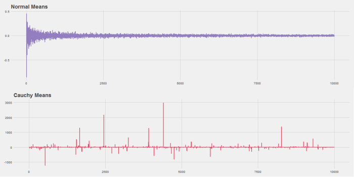
Notice that while the Normal distribution converges quickly the Cauchy never does. This is because the Cauchy distribution has fat tails and so extreme observations are common.
################################################################
# R Simulation
# James McCammon
# 2/20/2017
################################################################
# This script goes through the simulation of plotting both normal
# and Cauchy means for random vectors of size 1 to 10,000. It
# also demonstrates function creation and plotting.
# Highlight desired section and click "Run."

# Set working directory as needed
setwd("~/R Projects/All of Statistics")

###
# Calculate means and plot using base R
###

    # Set seed for reproducibility
    set.seed(271)

    #
    # Version 1: Simple
    #
    n = seq(from=1, to=10000, by=1)
    y=sapply(n, FUN=function(x) sum(rnorm(x))/x)
    plot(n, y, type="l")

    #
    # Version 2: Define a function
    #
    sim = function(x, FUN) {
      sapply(x, FUN=function(x) sum(FUN(x))/x)
    }

    # Use function to plot normal means
    x = seq(from=1, to=10000, by=1)
    y1 = sim(x, rnorm)
    plot(x, y1, type="l")

    # Use function to plot Cauchy means
    y2 = sim(x, rcauchy)
    plot(x, y2, type="l")

    #
    # Version 3: More complex function
    #

    # This function has:
    # (1) error checking
    # (2) extra argument options
    # (3) the ability to input any distribution R supports
    sim = function(x, FUN, ...) {
      if(!is.character(FUN)) stop('Please enter distribution as string.')
      dists = c('rnorm',
                'rbeta',
                'rbinom',
                'rcauchy',
                'rchisq',
                'rexp',
                'rf',
                'rgamma',
                'rgeom',
                'rhyper',
                'rlnorm',
                'rmultinom',
                'rnbinom',
                'rpois',
                'rt',
                'runif',
                'rweibull')
      if(is.na(match(FUN, dists))) stop(paste('Please enter a valid distribution from one of:', paste(dists, collapse=', ')))
      FUN = get(FUN)
      sapply(x, FUN=function(x) sum(FUN(x, ...))/x)
    }

    # We have to define our function in string form.
    # This will throw error 1.
    test1 = sim(x, rnorm)

    # We have to input a distribution R supports.
    # This will throw error 2.
    test2 = sim(x, 'my_cool_function')

    # We can input additional arguments like the
    # mean, standard deviations, or other shape parameters.
    test3 = sim(x, 'rnorm', mean=10, sd=2)

####
# Using ggplot2 to make pretty graph
###

    # Load libraries
    library(ggplot2)
    library(ggthemes)
    library(gridExtra)

    png(filename='Ch3-Pr9.png', width=1200, height=600)

      df1 = cbind.data.frame(x, y1)
      p1 = ggplot(df1, aes(x=x, y=y1)) +
        geom_line(size = 1, color='#937EBF') +
        theme_fivethirtyeight() +
        ggtitle("Normal Means")

      df2 = cbind.data.frame(x, y2)
      p2 = ggplot(df2, aes(x=x, y=y2)) +
        geom_line(size = 1, color='#EF4664') +
        theme_fivethirtyeight() +
        ggtitle("Cauchy Means")

      # Save charts
      grid.arrange(p1,p2,nrow=2,ncol=1)

    dev.off()
    # Print charts to screen
    grid.arrange(p1,p2,nrow=2,ncol=1)

 is irrational. An irrational number is one that cannot be written in the form
  , where
  and
and  are both integers; in other words there is no repeating pattern in it’s decimal.
 is a multiple of
  then so is
  . Then
  where
where  . Then
  . We can factor out a
  . This implies
  part). We have proved the contrapositive which implies our original proposition (
 is the same as
  ).
). with
with  which means
  . But this means
  is a multiple of
  . Let’s plug this in to get
  , simplifying we get that
  . Let’s divide through by
  . This means that
  is a multiple of
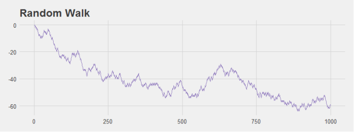
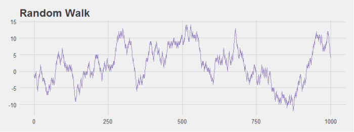

 and moves one unit to the left with probability
  and moves one unit to the right with probability
  . What is the expected position
 ![\mathbb{E}[X_n]](https://s0.wp.com/latex.php?latex=%5Cmathbb%7BE%7D%5BX_n%5D+&bg=ffffff&fg=000000&s=0&c=20201002) of the particle after
of the particle after 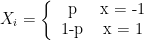

 . We can use rules of expected value to bring the expectation inside the summation and take the expectation of each individual
  as we normally would.
![\mathbb{E}[Y] = \mathbb{E}\big[\sum_{i=1}^{n} X_i \big]](https://s0.wp.com/latex.php?latex=%5Cmathbb%7BE%7D%5BY%5D+%3D+%5Cmathbb%7BE%7D%5Cbig%5B%5Csum_%7Bi%3D1%7D%5E%7Bn%7D+X_i+%5Cbig%5D+&bg=ffffff&fg=000000&s=0&c=20201002)
![\mathbb{E}[Y] = \sum_{i=1}^{n} \mathbb{E}[X_i]](https://s0.wp.com/latex.php?latex=%5Cmathbb%7BE%7D%5BY%5D+%3D+%5Csum_%7Bi%3D1%7D%5E%7Bn%7D+%5Cmathbb%7BE%7D%5BX_i%5D+&bg=ffffff&fg=000000&s=0&c=20201002)
![\mathbb{E}[Y] = \sum_{i=1}^{n} -1 \cdot p + 1 \cdot (1-p)](https://s0.wp.com/latex.php?latex=%5Cmathbb%7BE%7D%5BY%5D+%3D%C2%A0%5Csum_%7Bi%3D1%7D%5E%7Bn%7D+-1+%5Ccdot+p+%2B+1+%5Ccdot+%281-p%29+&bg=ffffff&fg=000000&s=0&c=20201002)
![\mathbb{E}[Y] = \sum_{i=1}^{n} 1 - 2p](https://s0.wp.com/latex.php?latex=%5Cmathbb%7BE%7D%5BY%5D+%3D+%C2%A0%5Csum_%7Bi%3D1%7D%5E%7Bn%7D+1+-+2p+&bg=ffffff&fg=000000&s=0&c=20201002)
![\mathbb{E}[Y] = n(1 - 2p)](https://s0.wp.com/latex.php?latex=%5Cmathbb%7BE%7D%5BY%5D+%3D+n%281+-+2p%29+&bg=ffffff&fg=000000&s=0&c=20201002)

![n=0: \quad \mathbb{E}[X_0] = z_i](https://s0.wp.com/latex.php?latex=n%3D0%3A+%5Cquad+%5Cmathbb%7BE%7D%5BX_0%5D+%3D+z_i+&bg=ffffff&fg=000000&s=0&c=20201002)
![n=1: \quad \mathbb{E}[X_1] = (z_i - 1)p + (z_i + 1)(1 - p)](https://s0.wp.com/latex.php?latex=n%3D1%3A+%5Cquad+%5Cmathbb%7BE%7D%5BX_1%5D+%3D+%28z_i+-+1%29p+%2B+%28z_i+%2B+1%29%281+-+p%29+&bg=ffffff&fg=000000&s=0&c=20201002)
![n=1: \quad \mathbb{E}[X_1] = z_{i}p - p + z_i + 1 - z_{i}p - p](https://s0.wp.com/latex.php?latex=n%3D1%3A+%5Cquad+%5Cmathbb%7BE%7D%5BX_1%5D+%3D+z_%7Bi%7Dp+-+p+%2B+z_i+%2B+1+-+z_%7Bi%7Dp+-+p+&bg=ffffff&fg=000000&s=0&c=20201002)
![n=1: \quad \mathbb{E}[X_1] = z_i + 1 - 2p](https://s0.wp.com/latex.php?latex=n%3D1%3A+%5Cquad+%5Cmathbb%7BE%7D%5BX_1%5D+%3D+z_i+%2B+1+-+2p+&bg=ffffff&fg=000000&s=0&c=20201002)
 our position is now the result from
  ,
,  .
.![n=2: \quad \mathbb{E}[X_2] = (z_i + 1 - 2p - 1)p + (z_i + 1 - 2p + 1)(1 - p)](https://s0.wp.com/latex.php?latex=n%3D2%3A+%5Cquad+%5Cmathbb%7BE%7D%5BX_2%5D+%3D+%28z_i+%2B+1+-+2p+-+1%29p+%2B+%28z_i+%2B+1+-+2p+%2B+1%29%281+-+p%29+&bg=ffffff&fg=000000&s=0&c=20201002)
![n=2: \quad \mathbb{E}[X_2] = z_{i}p - 2p^2 + Z_i - 2p + 2 - z_{i}p + 2p^2 - 2p](https://s0.wp.com/latex.php?latex=n%3D2%3A+%5Cquad+%5Cmathbb%7BE%7D%5BX_2%5D+%3D+z_%7Bi%7Dp+-+2p%5E2+%2B+Z_i+-+2p+%2B+2+-+z_%7Bi%7Dp+%2B+2p%5E2+-+2p&bg=ffffff&fg=000000&s=0&c=20201002)
![n=2: \quad \mathbb{E}[X_2] = z_i + 2(1 - 2p)](https://s0.wp.com/latex.php?latex=n%3D2%3A+%5Cquad+%5Cmathbb%7BE%7D%5BX_2%5D+%3D+z_i+%2B+2%281+-+2p%29+&bg=ffffff&fg=000000&s=0&c=20201002)
![\mathbb{E}[X_n] = z_i + n(1 - 2p)](https://s0.wp.com/latex.php?latex=%5Cmathbb%7BE%7D%5BX_n%5D+%3D+z_i+%2B+n%281+-+2p%29+&bg=ffffff&fg=000000&s=0&c=20201002) . But we can prove this formally through induction. We’ve already done our base case, so let’s now do the induction step. We will assume that
. But we can prove this formally through induction. We’ve already done our base case, so let’s now do the induction step. We will assume that  .
.![\mathbb{E}[X_{n+1}] = (z_i + n(1 - 2p) - 1)p + (z_i + n(1 - 2p) + 1)(1 - p)](https://s0.wp.com/latex.php?latex=%5Cmathbb%7BE%7D%5BX_%7Bn%2B1%7D%5D+%3D+%28z_i+%2B+n%281+-+2p%29+-+1%29p+%2B+%28z_i+%2B+n%281+-+2p%29+%2B+1%29%281+-+p%29&bg=ffffff&fg=000000&s=0&c=20201002)
![\mathbb{E}[X_{n+1}] = (z_i + n - 2pn - 1)p + (z_i + n - 2pn + 1)(1 - p)](https://s0.wp.com/latex.php?latex=%5Cmathbb%7BE%7D%5BX_%7Bn%2B1%7D%5D+%3D+%28z_i+%2B+n+-+2pn+-+1%29p+%2B+%28z_i+%2B+n+-+2pn+%2B+1%29%281+-+p%29&bg=ffffff&fg=000000&s=0&c=20201002)
![\mathbb{E}[X_{n+1}] = z_{i}p + pn - 2p^{2}n - p + z_i + n - 2pn + 1 -z_{i}p - pn + 2p^{2}n - p](https://s0.wp.com/latex.php?latex=%5Cmathbb%7BE%7D%5BX_%7Bn%2B1%7D%5D+%3D+z_%7Bi%7Dp+%2B+pn+-+2p%5E%7B2%7Dn+-+p+%2B+z_i+%2B+n+-+2pn+%2B+1+-z_%7Bi%7Dp+-+pn+%2B+2p%5E%7B2%7Dn+-+p+&bg=ffffff&fg=000000&s=0&c=20201002)
![\mathbb{E}[X_{n+1}] = - p + z_i + n - 2pn + 1 - p](https://s0.wp.com/latex.php?latex=%5Cmathbb%7BE%7D%5BX_%7Bn%2B1%7D%5D+%3D+-+p+%2B+z_i+%2B+n+-+2pn+%2B+1+-+p+&bg=ffffff&fg=000000&s=0&c=20201002)
![\mathbb{E}[X_{n+1}] = z_i + (n + 1)(1 - 2p)](https://s0.wp.com/latex.php?latex=%5Cmathbb%7BE%7D%5BX_%7Bn%2B1%7D%5D+%3D+z_i+%2B+%28n+%2B+1%29%281+-+2p%29+&bg=ffffff&fg=000000&s=0&c=20201002)
![\mathbb{E}[X_n] = n(1 - 2p)](https://s0.wp.com/latex.php?latex=%5Cmathbb%7BE%7D%5BX_n%5D+%3D+n%281+-+2p%29+&bg=ffffff&fg=000000&s=0&c=20201002) .
. . This would mean we have an equal chance of moving left or moving right. Over the long run we would expect our final position to be exactly where we started. Plugging in
  . Just as we expected! What if
  ? This means we only move to the left. Plugging
  . This makes sense! If we can only move to the left then after