
Let’s do a problem from Chapter 5 of All of Statistics.
Suppose 


Note that we have

Recall from Theorem 5.5(e) that if 


So the question becomes does 


![\bar{X}_n \overset{P}{\longrightarrow} \mathbb{E}[X]](https://s0.wp.com/latex.php?latex=%5Cbar%7BX%7D_n+%5Coverset%7BP%7D%7B%5Clongrightarrow%7D+%5Cmathbb%7BE%7D%5BX%5D+&bg=ffffff&fg=000000&s=0&c=20201002)

![\mathbb{E}[X] = .5](https://s0.wp.com/latex.php?latex=%5Cmathbb%7BE%7D%5BX%5D+%3D+.5+&bg=ffffff&fg=000000&s=0&c=20201002)
Putting it all together we have that:
![Y_n \rightsquigarrow \mathbb{E}[X]\mathbb{E}[X]](https://s0.wp.com/latex.php?latex=Y_n+%5Crightsquigarrow+%5Cmathbb%7BE%7D%5BX%5D%5Cmathbb%7BE%7D%5BX%5D+&bg=ffffff&fg=000000&s=0&c=20201002)


We can also show this by simulation in R, which produces this chart:
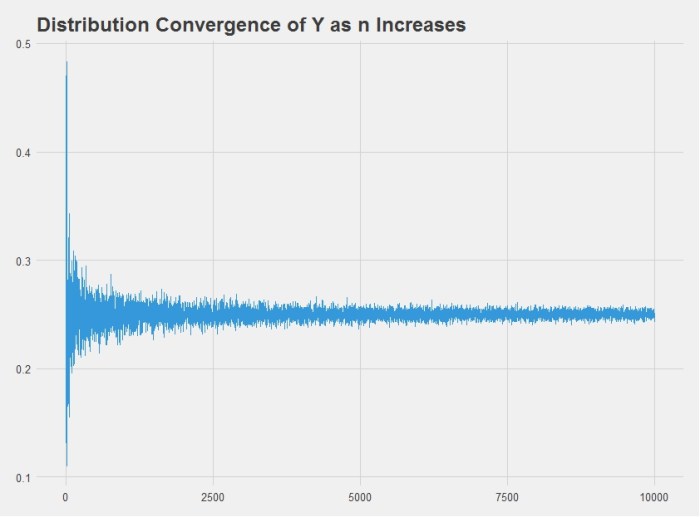
Indeed we also get the answer 0.25. Here is the R code used to produce the chart above:
# Load plotting libraries
library(ggplot2)
library(ggthemes)

# Create Y = g(x_n)
g = function(n) {
  return(mean(runif(n))^2)
}

# Define variables
n = 1:10000
Y = sapply(n, g)

# Plot
set.seed(10)
df = data.frame(n,Y)
ggplot(df, aes(n,Y)) +
  geom_line(color='#3498DB') +
  theme_fivethirtyeight() +
  ggtitle('Distribution Convergence of Y as n Increases')
